Chapter 4 Summary Statistics

Now that we have filtered and cleaned the data, and created the Range and sampling Events tables for zero-filling the data matrix, we are ready to start generating summary statistics. These summary statistics are generated annually to support Birds Canada’s reporting for Canadian PFW participants.

Let’s start this Chapter by reloading our libraries and resetting our working directories in the event you took a break and are starting a new session with your newly filtered and cleaned data set.

require(tidyverse)
require(data.table)

out.dir <- paste("Output/")
dat.dir <- paste("Data/")

# Load full dataset
data<-fread("Data/PFW_Canada_All.csv")

Before we proceed we are going to add one more filter to the data. Specifically, there are some CATEGORY types that are not useful for our summary purposes (e.g., hybrids = slash & integrade, unknown = spuh, undescribed = form, and domestic = domestic).

If you want to keep all records, then skip this step.

data<-data %>% filter(CATEGORY %in% c("species", "issf")) %>% droplevels() 

4.1 Average number of birds per week

Calculate the average number of individual birds per week at each station, summarized by region, province and nationally.

Note that this is not a zero-filled data matrix. I assume that all checklists have a minimum of one bird recorded. This is likely a true assumption.

# Region
ind.week.reg<-data %>% group_by(region, Period, floor.week, loc_id) %>% 
  summarize(loc.sum=sum(how_many))

ind.week.reg<-ind.week.reg %>% group_by(region, Period) %>% 
  summarize(reg.ave=mean(loc.sum))  
  
ind.week.region<-cast(ind.week.reg, Period~region, value="reg.ave")

write.table(format(ind.week.region, digits=4), file = paste(out.dir,"Average number of individual birds per week_region.csv"), row.names = FALSE, col.name = TRUE, append = FALSE, quote = FALSE, sep = ",")

# Province
ind.week.prov<-data %>% group_by(Prov, Period, floor.week, loc_id) %>%   summarize(loc.sum=sum(how_many))

ind.week.prov<-ind.week.prov %>% group_by(Prov, Period) %>% 
  summarize(prov.ave=mean(loc.sum))  
  
ind.week.province<-cast(ind.week.prov, Period~Prov, value="prov.ave")

write.table(format(ind.week.province, digits=4), file = paste(out.dir,"Average number of individual birds per week_province.csv"), row.names = FALSE, col.name = TRUE, append = FALSE, quote = FALSE, sep = ",")

# National
ind.week.nat <-data %>% group_by(Period, floor.week, loc_id) %>% summarize(loc.sum=sum(how_many))

ind.week.nat<-ind.week.nat %>% group_by(Period) %>% 
  summarize(nat.ave=mean(loc.sum))

ind.week.nat<-as.data.frame((ind.week.nat))
  
write.table(format(ind.week.nat, digits=4), file = paste(out.dir,"Average number of individual birds per week_national.csv"), row.names = FALSE, col.name = TRUE, append = FALSE, quote = FALSE, sep = ",")

4.2 Average number of species per week

Calculate the average number of species (REPORT_AS) per week at each station, summarized by region, province and nationally.

Note that this is not a zero-filled data matrix. I assume that all checklists have a minimum of one bird recorded. This is likely a true assumption.

# Region
sp.week.reg<-data %>% group_by(region, Period, floor.week, loc_id) %>% 
  summarize(loc.sp=n_distinct(REPORT_AS))
 
sp.week.reg<-sp.week.reg %>% group_by(region, Period) %>% 
  summarize(reg.ave=mean(loc.sp))

sp.week.reg<-cast(sp.week.reg, Period~region, value="reg.ave")

write.table(format(sp.week.reg, digits=3), file = paste(out.dir,"Average number of species per week_region.csv"), row.names = FALSE, col.name = TRUE, append = FALSE, quote = FALSE, sep = ",")

# Province
sp.week.prov<-data %>% group_by(Prov, Period, floor.week, loc_id) %>% 
  summarize(loc.sp=n_distinct(REPORT_AS))
 
sp.week.prov<-sp.week.prov %>% group_by(Prov, Period) %>% summarize(prov.ave=mean(loc.sp))

sp.week.prov<-cast(sp.week.prov, Period~Prov, value="prov.ave")

write.table(format(sp.week.prov, digits=3), file = paste(out.dir,"Average number of species per week_province.csv"), row.names = FALSE, col.name = TRUE, append = FALSE, quote = FALSE, sep = ",")

# National
sp.week.nat<-data %>% group_by(Period, floor.week, loc_id) %>% 
  summarize(loc.sp=n_distinct(REPORT_AS))
 
sp.week.nat<-sp.week.nat %>% group_by(Period) %>% summarize(nat.ave=mean(loc.sp))

sp.week.nat<-as.data.frame((sp.week.nat))

write.table(format(sp.week.nat, digits=3), file = paste(out.dir,"Average number of species per week_national.csv"), row.names = FALSE, col.name = TRUE, append = FALSE, quote = FALSE, sep = ",")

These number are inflated because there are species in the list that are not strictly feeder birds.

4.3 Average number of species per site

Calculate the average number of species (REPORT_AS) per site in total years (all weeks combined) summarized by region, province and nationally.

Note that this is not a zero-filled data matrix. I assume that all checklists have a minimum of one bird recorded. This is likely a true assumption.

# Region
tot.sp<-data %>% group_by(loc_id, Period, region) %>% 
  summarise(mean.sp.site=n_distinct(REPORT_AS)) %>% 
  group_by(Period, region) %>% 
  summarise(mean.sp=mean(mean.sp.site))

tot.sp<-cast(tot.sp, Period~region, value="mean.sp")

write.table(format(tot.sp, digits=3), file = paste(out.dir,"Average number of species per site in total years_region.csv"), row.names = FALSE, col.name = TRUE, append = FALSE, quote = FALSE, sep = ",")

# Province
tot.sp.prov<-data %>% group_by(loc_id, Period, Prov) %>% 
  summarise(mean.sp.site=n_distinct(REPORT_AS)) %>% 
  group_by(Period, Prov) %>% 
  summarise(mean.sp=mean(mean.sp.site))

tot.sp.prov<-cast(tot.sp.prov, Period~Prov, value="mean.sp")

write.table(format(tot.sp.prov, digits=3), file = paste(out.dir,"Average number of species per site in total years_province.csv"), row.names = FALSE, col.name = TRUE, append = FALSE, quote = FALSE, sep = ",")

# National
tot.sp.nat<-data %>% group_by(loc_id, Period) %>% 
  summarise(mean.sp.site=n_distinct(REPORT_AS)) %>% 
  group_by(Period) %>% 
  summarise(mean.sp=mean(mean.sp.site))

tot.sp.nat<-as.data.frame((tot.sp.nat))

write.table(format(tot.sp.nat, digits=3), file = paste(out.dir,"Average number of species per site in total years_national.csv"), row.names = FALSE, col.name = TRUE, append = FALSE, quote = FALSE, sep = ",")

These numbers may be slightly inflated because there are species in the list that are not strictly feeder birds.

4.4 Average group size when the species is present

This summary statistic captures the geometric mean group size of species for sites and year when it is present. It is therefore not a zero-filled data matrix.

# define the geometric mean function
gmean <- function(x) exp(mean(log(x)))

# Region
nsite<-data %>% group_by(Period, region) %>%   summarize(nloc=n_distinct(loc_id)) %>% filter(nloc>=10)  %>% dplyr::select(-nloc)
  
mean.sp<-right_join(data, nsite, by=c("Period", "region")) 

mean.sp<-mean.sp %>% group_by(Period, region, REPORT_AS) %>% summarise(mean.group=gmean(how_many))

mean.sp<-cast(mean.sp, REPORT_AS+region~Period, value="mean.group")

write.table(format(mean.sp, digits=3), file = paste(out.dir,"Mean group size of species_region.csv"), row.names = FALSE, col.name = TRUE, append = FALSE, quote = FALSE, sep = ",")

# Provincial 
nsite<-data %>% group_by(Period, Prov) %>%   summarize(nloc=n_distinct(loc_id)) %>% filter(nloc>=10)  %>% dplyr::select(-nloc)
  
mean.sp<-right_join(data, nsite, by=c("Period", "Prov")) 

mean.sp<-mean.sp %>% group_by(Period, Prov, REPORT_AS) %>% summarise(mean.group=gmean(how_many))

mean.sp<-cast(mean.sp, REPORT_AS+region~Period, value="mean.group")

write.table(format(mean.sp, digits=3), file = paste(out.dir,"Mean group size of species_prov.csv"), row.names = FALSE, col.name = TRUE, append = FALSE, quote = FALSE, sep = ",")

# National
nsite<-data %>% group_by(Period) %>%   summarize(nloc=n_distinct(loc_id)) %>% filter(nloc>=10) %>% dplyr::select(-nloc)
  
mean.sp<-right_join(data, nsite, by=c("Period")) 

mean.sp<-mean.sp %>% group_by(Period, REPORT_AS) %>% summarise(mean.group=gmean(how_many))

mean.sp<-cast(mean.sp, REPORT_AS~Period, value="mean.group")

write.table(format(mean.sp, digits=3), file = paste(out.dir,"Mean group size of species_national.csv"), row.names = FALSE, col.name = TRUE, append = FALSE, quote = FALSE, sep = ",")

4.5 Percent of sites with species at least once and mean group size

Now we will do something a little more complicated: calculate the percent of sites with species (REPORT_AS) at least once in a season and mean group size. This is calculated for species that occur at > 10 feeder sites.

This summary statistics needs to be done on a zero-fill data matrix to correct for the number of sites an individual could have been seen but was not. To do this, we will use the Range_prov or Range_blockcode table, and the sampling Events table (see Chapter 3).

# Region
# Create regional table outside loop
per.site.region<- as.data.frame(matrix(data = NA, nrow = 1, ncol = 5, byrow = FALSE, dimnames = NULL))
names(per.site.region) <- c("Region", "Period", "MeanGroup", "PercentSite", "Species")
write.table(per.site.region, file = paste(out.dir,"% sites with species at least once in season and mean group size_region.csv"), row.names = FALSE, append = FALSE, quote = FALSE, sep = ",")

# Read in your tables from the Output folder
range<-fread("Output/Range_prov.csv") 
range<-data.frame(range)
events<-fread("Output/Events.csv")

sp.list<-unique(data$REPORT_AS)

# Regional species loop 
for(n in 1:length(sp.list)) {
  
   # n<-1 #for testing each species

events1<-NULL #clear previous dataframe
events1<-events %>% dplyr::select(loc_id, sub_id, day, month, year, Period, Prov, region)%>% filter(year!="NA") 

  sp.data <-NULL #clear previous dataframe
  sp.data <- filter(data, REPORT_AS == sp.list[n]) %>%
      droplevels()

  if(nrow(sp.data)>0){ #only continue if there is data
  
min.year<-min(sp.data$year)
max.year<-max(sp.data$year)  
  
# Filter events data using the sp.data min and max year
events1<-events1 %>% filter(year>=min.year & year<=max.year)
  
# Merge sp.data to events data
sp.data<-dplyr::left_join(events1, sp.data, by=c("loc_id", "sub_id", "day", "month", "year", "Period", "Prov", "region"))
sp.data<-sp.data %>% filter(loc_id != "NA") 
  
range.data<-NULL #clear previous dataframe
range.data<-try(range %>% dplyr::select(Prov, sp.list[n]), silent=T) 

if(class(range.data) !="try-error"){
  
# Join tables
  sp.data<-left_join(sp.data, range.data, by="Prov")
  
#remove blocks that should not be included in the zero count
  colnames(sp.data)[colnames(sp.data) == sp.list[n]] <- "sp"
  sp.data<-sp.data %>% filter(sp>=1)
  
# Zero fill the 'how_many' column
  sp.data$how_many[is.na(sp.data$how_many)] <- 0 
   
# Now we can start building the summary statistics

# Determine the number of distinct locations and the mean group size each location 
# Filter the data to include only species that have at least once per site, and seen at > 10 sites. 
per.site.region<-sp.data %>% group_by(region, Period) %>% 
mutate(loc_id_sp = ifelse(how_many==0, NA, loc_id)) %>%
summarize(tot.site=n_distinct(loc_id), n.site.sp=n_distinct(loc_id_sp), sp.sum=sum(how_many), mean.group=mean(how_many)) %>% filter(sp.sum > 0) %>% filter(tot.site>=10) %>% mutate(per.site=((n.site.sp-1)/tot.site)*100) %>% #subtract 1 for NAs
    dplyr::select(-sp.sum, -n.site.sp, -tot.site)

  per.site.region$SpeciesCode<-sp.list[n]
  per.site.region<-as.data.frame(per.site.region)

write.table(format(per.site.region, digits=3), file = paste(out.dir,"% sites with species at least once in season and mean group size_region.csv"), row.names = FALSE, col.name = FALSE, append = TRUE, quote = FALSE, sep = ",")
 
} # end try catch 
  } # end if nrow>0
    } #end species loop

########################################

# Province
# Create provincial table outside loop
per.site.prov<- as.data.frame(matrix(data = NA, nrow = 1, ncol = 5, byrow = FALSE, dimnames = NULL))
names(per.site.prov) <- c("Prov", "Period", "MeanGroup", "PercentSite", "Species")
write.table(per.site.prov, file = paste(out.dir,"% sites with species at least once in season and mean group size_prov.csv"), row.names = FALSE, append = FALSE, quote = FALSE, sep = ",")

range<-fread("Output/Range_prov.csv")
range<-data.frame(range)
events<-fread("Output/Events.csv")

sp.list<-unique(data$REPORT_AS)

# Provincial species loop

for(n in 1:length(sp.list)) {
  
   # n<-1 #for testing each species

events1<-NULL #clear previous dataframe
events1<-events %>% dplyr::select(loc_id, sub_id, day, month, year, Period, Prov, region)%>% filter(year!="NA") 

  sp.data <-NULL 
  sp.data <- filter(data, REPORT_AS == sp.list[n]) %>%
      droplevels()

  if(nrow(sp.data)>0){ #only continue if there is data
  
min.year<-min(sp.data$year)
max.year<-max(sp.data$year)  
  
# Filter events data using the sp.data min and max year
events1<-events1 %>% filter(year>=min.year & year<=max.year)
  
# First merge to events data
sp.data<-dplyr::left_join(events1, sp.data, by=c("loc_id", "sub_id", "day", "month", "year", "Period", "Prov", "region"))
sp.data<-sp.data %>% filter(loc_id != "NA") 

  range.data<-NULL

# Some oddly labeled species are not in the block list. We therefore need a trycath to catch these errors so that the loop doesn't get broken.     
  range.data<-try(range %>% dplyr::select(Prov, sp.list[n]), silent=TRUE)
  
if(class(range.data) !="try-error"){
  
# Join tables
  sp.data<-left_join(sp.data, range.data, by="Prov")
  
# Remove blocks that should not be included in the zero count
  colnames(sp.data)[colnames(sp.data) == sp.list[n]] <- "sp"
  sp.data<-sp.data %>% filter(sp>=1)
  
# Zero fill the 'how_many' column
  sp.data$how_many[is.na(sp.data$how_many)] <- 0 
   
# Now we can start building the summary statistics

# Determine the number of distinct locations and the mean group size each location  
  per.site.prov<-sp.data %>% group_by(Prov, Period) %>% 
mutate(loc_id_sp = ifelse(how_many==0, NA, loc_id)) %>%
summarize(tot.site=n_distinct(loc_id), n.site.sp=n_distinct(loc_id_sp), sp.sum=sum(how_many), mean.group=mean(how_many)) %>% filter(sp.sum > 0) %>% filter(tot.site>=10) %>% mutate(per.site=((n.site.sp-1)/tot.site)*100) %>% #subtract 1 for NAs
    dplyr::select(-sp.sum, -n.site.sp, -tot.site)

  per.site.prov$SpeciesCode<-sp.list[n]
  per.site.prov<-as.data.frame(per.site.prov)

write.table(format(per.site.prov, digits=3), file = paste(out.dir,"% sites with species at least once in season and mean group size_prov.csv"), row.names = FALSE, col.name = FALSE, append = TRUE, quote = FALSE, sep = ",")

} #end try catch
  } # end if nrow>0
    } #end species loop

########################################
# National

# Create provincial table outside loop
per.site.nat<- as.data.frame(matrix(data = NA, nrow = 1, ncol = 4, byrow = FALSE, dimnames = NULL))
names(per.site.nat) <- c("Period", "MeanGroup", "PercentSite", "Species")
write.table(per.site.nat, file = paste(out.dir,"% sites with species at least once in season and mean group size_nat.csv"), row.names = FALSE, append = FALSE, quote = FALSE, sep = ",")

range<-fread("Output/Range_prov.csv")
range<-data.frame(range)
events<-fread("Output/Events.csv")

sp.list<-unique(data$REPORT_AS)

# Provincial species loop

for(n in 1:length(sp.list)) {
  
   # n<-1 #for testing each species
  
events1<-NULL #clear previous dataframe
events1<-events %>% dplyr::select(loc_id, sub_id, day, month, year, Period, Prov, region)%>% filter(year!="NA")

  sp.data <-NULL 
  sp.data <- filter(data, REPORT_AS == sp.list[n]) %>%
      droplevels()

  if(nrow(sp.data)>0){ #only continue if there is data
  
min.year<-min(sp.data$year)
max.year<-max(sp.data$year)  
  
# Filter events data using the sp.data min and max year
events1<-events1 %>% filter(year>=min.year & year<=max.year)
  
# First merge to events data
sp.data<-dplyr::left_join(events1, sp.data, by=c("loc_id", "sub_id", "day", "month", "year", "Period", "Prov", "region"))
sp.data<-sp.data %>% filter(loc_id != "NA") 
  
  range.data<-NULL
  range.data<-try(range %>% dplyr::select(Prov, sp.list[n]), silent=T)
  
if(class(range.data) !="try-error"){
  
# Join tables
  sp.data<-left_join(sp.data, range.data, by="Prov")
  
# Remove blocks that should not be included in the zero count
  colnames(sp.data)[colnames(sp.data) == sp.list[n]] <- "sp"
  sp.data<-sp.data %>% filter(sp>=1)
  
# Zero fill the 'how_many' column
  sp.data$how_many[is.na(sp.data$how_many)] <- 0 
   
# Now we can start building the summary statistics

# Determine the number of distinct locations and the mean group size each location  
  per.site.nat<-sp.data %>% group_by(Period) %>% 
mutate(loc_id_sp = ifelse(how_many==0, NA, loc_id)) %>%
summarize(tot.site=n_distinct(loc_id), n.site.sp=n_distinct(loc_id_sp), sp.sum=sum(how_many), mean.group=mean(how_many)) %>% filter(sp.sum > 0) %>% filter(tot.site>=10) %>% mutate(per.site=((n.site.sp-1)/tot.site)*100) %>% #subtract 1 for NAs
    dplyr::select(-sp.sum, -n.site.sp, -tot.site)

  per.site.nat$SpeciesCode<-sp.list[n]
  per.site.nat<-as.data.frame(per.site.nat)

write.table(format(per.site.nat, digits=3), file = paste(out.dir,"% sites with species at least once in season and mean group size_nat.csv"), row.names = FALSE, col.name = FALSE, append = TRUE, quote = FALSE, sep = ",")
  
} #end try catch
  } # end if nrow>0
    } #end species loop

4.6 Top 10 Species

The last summary statistic we will derive is the Top 10 Species each year based on the % of feeders and the mean group size, separately. To do this, we will use the output tables from the previous analysis.

# Load the tables if they are not in your working environment

per.site.region<-read.csv("Output/ % sites with species at least once in season and mean group size_region.csv")
  
per.site.prov<-read.csv("Output/ % sites with species at least once in season and mean group size_prov.csv")
  
per.site.nat<-read.csv("Output/ % sites with species at least once in season and mean group size_nat.csv")

# Top 10 species based on % feeders
# Region
top10.per.reg<-per.site.region %>% dplyr::select(-MeanGroup) %>% group_by(Period, Region) %>% slice_max(order_by = PercentSite, n = 10) 
top10.per.reg<-as.data.frame(top10.per.reg)

write.table(format(top10.per.reg, digits=3), file = paste(out.dir,"Top 10 species percent feeders_region.csv"), row.names = FALSE, col.name = TRUE, append = FALSE, quote = FALSE, sep = ",")

# Prov
top10.per.prov<-per.site.prov %>% dplyr::select(-MeanGroup) %>% group_by(Period, Prov) %>% slice_max(order_by = PercentSite, n = 25) 
top10.per.prov<-as.data.frame(top10.per.prov)

write.table(format(top10.per.prov, digits=3), file = paste(out.dir,"Top 10 species percent feeders_prov.csv"), row.names = FALSE, col.name = TRUE, append = FALSE, quote = FALSE, sep = ",")

# National 
top10.per.nat<-per.site.nat %>% dplyr::select(-MeanGroup) %>% group_by(Period) %>% slice_max(order_by = PercentSite, n = 10) 
top10.per.nat<-as.data.frame(top10.per.nat)

write.table(format(top10.per.nat, digits=3), file = paste(out.dir,"Top 10 species percent feeders_nat.csv"), row.names = FALSE, col.name = TRUE, append = FALSE, quote = FALSE, sep = ",")

# Top 10 species based on MeanGroup size
# Region
top10.mean.reg<-per.site.region %>% dplyr::select(-PercentSite) %>% group_by(Period, Region) %>% slice_max(order_by = MeanGroup, n = 10) 
top10.mean.reg<-as.data.frame(top10.mean.reg)

write.table(format(top10.mean.reg, digits=3), file = paste(out.dir,"Top 10 species mean group feeders_region.csv"), row.names = FALSE, col.name = TRUE, append = FALSE, quote = FALSE, sep = ",")

# Prov
top10.mean.prov<-per.site.prov %>% dplyr::select(-PercentSite) %>% group_by(Period, Prov) %>% slice_max(order_by = MeanGroup, n = 10) 
top10.mean.prov<-as.data.frame(top10.mean.prov)

write.table(format(top10.mean.prov, digits=3), file = paste(out.dir,"Top 10 species mean group feeders_prov.csv"), row.names = FALSE, col.name = TRUE, append = FALSE, quote = FALSE, sep = ",")

# National 
top10.mean.nat<-per.site.nat %>% dplyr::select(-PercentSite) %>% group_by(Period) %>% slice_max(order_by = MeanGroup, n = 10) 
top10.mean.nat<-as.data.frame(top10.mean.nat)

write.table(format(top10.mean.nat, digits=3), file = paste(out.dir,"Top 10 species mean group feeders_nat.csv"), row.names = FALSE, col.name = TRUE, append = FALSE, quote = FALSE, sep = ",")

4.7 Plot Species Means

Now that we have generated the datatables, let’s plot some data of interest.

First, lets look at changes in the mean number of species over time. This can be done regionally, provincially, and/ or nationally with only slight changes to the code below. Also, you can simply change the filter to whichever species you want to plot over time.

Notice that the REPORT_AS is now labled as Species in the output tables.

# Load the tables if they are not in your working environment
per.site.region<-read.csv("Output/ % sites with species at least once in season and mean group size_region.csv")
  
per.site.prov<-read.csv("Output/ % sites with species at least once in season and mean group size_prov.csv")
  
per.site.nat<-read.csv("Output/ % sites with species at least once in season and mean group size_nat.csv")


# Filter for the species of interest 
sp.mean<-per.site.region %>% filter(Species=="amecro")

# Plot the mean number
ggplot(sp.mean, aes(Period, MeanGroup))+
  geom_line(aes(colour=Region), size=1)+
  theme_classic()+
  theme(text=element_text(size=20))+
  ylab("Mean number per site")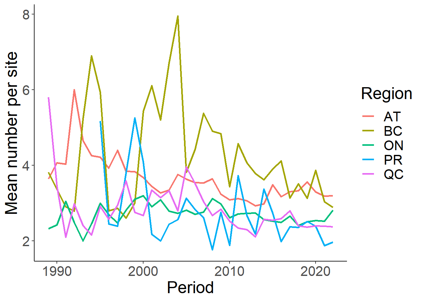

# Plot the % feeders 
ggplot(sp.mean, aes(Period, PercentSite))+
  geom_line(aes(colour=Region), size=1)+
  theme_classic()+
  theme(text=element_text(size=20))+
  ylab("% feeder sites")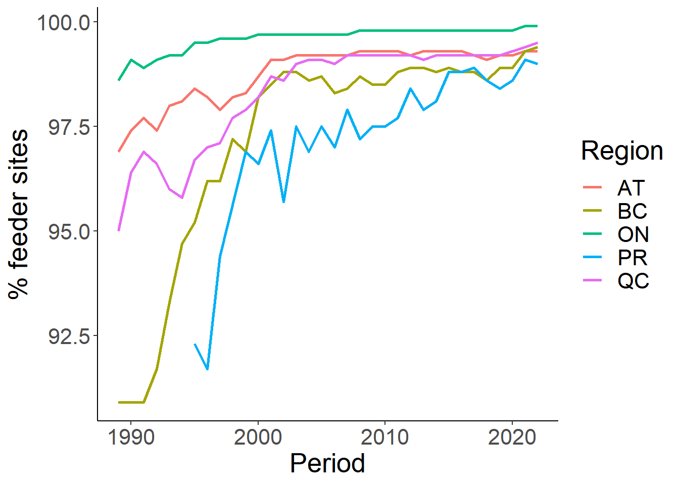

Next we are going to summarize effort in Chapter 5.