Mapping Observations
2026-03-31
Source:vignettes/articles/mapping-observations.Rmd
mapping-observations.RmdIn this article we’ll walk through how to create various types of
maps of the observations downloaded with naturecounts to
get a sense of the spatial distribution.
The following examples use the “testuser” user which is not available to you. You can quickly sign up for a free account of your own to access and play around with these examples. Simply replace
testuserwith your own username.
Setup
To do so we’re going to use the following packages:
library(naturecounts)
library(sf)
library(rnaturalearth)
library(ggplot2)
library(ggspatial)
library(dplyr)
library(tidyr)
library(mapview)
First we’ll use download some data:
house_finches <- nc_data_dl(
  species = 20350,
  region = list(statprov = "AB"),
  username = "testuser",
  info = "nc_tutorial"
)
## The server did not respond within 30s. Trying again...## Using filters: species (20350); fields_set (BMDE2.00-ext); statprov (AB)## Collecting available records...## collection nrecords
## 1 ABATLAS1 5
## 2 ABATLAS2 202
## 3 ABBIRDRECS 4
## 4 BBL-1990-1999 13
## 5 BBL-2000-2009 978
## 6 BBL-2010-2019 1299
## ...
## Total records: 11,061##
## Downloading records for each collection:## ABATLAS1## Records 1 to 5 / 5## ABATLAS2## Records 1 to 202 / 202## ABBIRDRECS## Records 1 to 4 / 4## BBL-1990-1999## Records 1 to 13 / 13## BBL-2000-2009## Records 1 to 978 / 978## BBL-2010-2019## Records 1 to 1299 / 1299## BBL-2020-2029## Records 1 to 51 / 51## BBS## Records 1 to 14 / 14## GBIF_50C9509D## Records 1 to 799 / 799## GBIF_6AC3F774## Records 1 to 1 / 1## GBIF_8A863029## Records 1 to 19 / 19## GBIF_B1047888## Records 1 to 2 / 2## PFW## Records 1 to 5000 / 7665## Records 5001 to 7665 / 7665## WILDTRAX1## Records 1 to 7 / 7## WILDTRAX19## Records 1 to 1 / 1## WILDTRAX41## Records 1 to 1 / 1
head(house_finches)## record_id collection project_id protocol_id protocol_type species_id
## 1 225655455 ABATLAS1 1048 NA NA 20350
## 2 225665275 ABATLAS1 1048 NA NA 20350
## 3 225690982 ABATLAS1 1048 NA NA 20350
## 4 225691486 ABATLAS1 1048 NA NA 20350
## 5 225691588 ABATLAS1 1048 NA NA 20350
## 6 225102049 ABATLAS2 1048 NA NA 20350
## statprov_code country_code SiteCode latitude longitude bcr subnational2_code
## 1 AB CA 4156 50.03028 -113.5828 11 CA.AB.03
## 2 AB CA 5307 49.87333 -112.1828 11 CA.AB.02
## 3 AB CA 1112 52.84139 -118.1128 10 CA.AB.15
## 4 AB CA 1112 52.84139 -118.1128 10 CA.AB.15
## 5 AB CA 1112 52.84139 -118.1128 10 CA.AB.15
## 6 AB CA 11268 50.05764 -110.6520 11 CA.AB.01
## iba_site utm_square survey_year survey_month survey_week survey_day
## 1 N/A 12UUA14 1990 8 2 9
## 2 N/A 12UVA12 1989 1 1 1
## 3 N/A 11UMU25 1988 5 2 14
## 4 N/A 11UMU25 1988 5 2 14
## 5 N/A 11UMU25 1988 6 4 27
## 6 N/A 12UWA24 2001 12 2 16
## breeding_rank GlobalUniqueIdentifier DateLastModified
## 1 0 URN:NatureAlberta:ABATLAS1:A4101-HOFI Jun 23 2015 6:49PM
## 2 0 URN:NatureAlberta:ABATLAS1:B3021-HOFI Jun 23 2015 6:49PM
## 3 10 URN:NatureAlberta:ABATLAS1:F2021-HOFI Jun 23 2015 6:49PM
## 4 10 URN:NatureAlberta:ABATLAS1:F2066-HOFI Jun 23 2015 6:49PM
## 5 10 URN:NatureAlberta:ABATLAS1:F2055-HOFI Jun 23 2015 6:49PM
## 6 0 URN:NatureAlberta:ABATLAS2:3986-HOFI Jun 23 2015 4:00PM
## BasisOfRecord InstitutionID InstitutionCode CollectionCode CatalogNumber
## 1 Observation NA NatureAlberta ABATLAS1 A4101-HOFI
## 2 Observation NA NatureAlberta ABATLAS1 B3021-HOFI
## 3 Observation NA NatureAlberta ABATLAS1 F2021-HOFI
## 4 Observation NA NatureAlberta ABATLAS1 F2066-HOFI
## 5 Observation NA NatureAlberta ABATLAS1 F2055-HOFI
## 6 Observation NA NatureAlberta ABATLAS2 3986-HOFI
## ScientificName HigherTaxon Kingdom
## 1 Haemorhous mexicanus AnimaliaChordataAvesPasseriformesFringillidae Animalia
## 2 Haemorhous mexicanus AnimaliaChordataAvesPasseriformesFringillidae Animalia
## 3 Haemorhous mexicanus AnimaliaChordataAvesPasseriformesFringillidae Animalia
## 4 Haemorhous mexicanus AnimaliaChordataAvesPasseriformesFringillidae Animalia
## 5 Haemorhous mexicanus AnimaliaChordataAvesPasseriformesFringillidae Animalia
## 6 Haemorhous mexicanus AnimaliaChordataAvesPasseriformesFringillidae Animalia
## Phylum Class OrderTaxon Family Genus SpecificEpithet
## 1 Chordata Aves Passeriformes Fringillidae Haemorhous mexicanus
## 2 Chordata Aves Passeriformes Fringillidae Haemorhous mexicanus
## 3 Chordata Aves Passeriformes Fringillidae Haemorhous mexicanus
## 4 Chordata Aves Passeriformes Fringillidae Haemorhous mexicanus
## 5 Chordata Aves Passeriformes Fringillidae Haemorhous mexicanus
## 6 Chordata Aves Passeriformes Fringillidae Haemorhous mexicanus
## InfraspecificRank InfraspecificEpithet ScientificNameAuthor
## 1 Subspecies <NA> NA
## 2 Subspecies <NA> NA
## 3 Subspecies <NA> NA
## 4 Subspecies <NA> NA
## 5 Subspecies <NA> NA
## 6 Subspecies <NA> NA
## IdentificationQualifier HigherGeography Continent WaterBody IslandGroup
## 1 NA <NA> NorthAmerica NA NA
## 2 NA <NA> NorthAmerica NA NA
## 3 NA <NA> NorthAmerica NA NA
## 4 NA <NA> NorthAmerica NA NA
## 5 NA <NA> NorthAmerica NA NA
## 6 NA <NA> NorthAmerica NA NA
## Island Country StateProvince County Locality
## 1 NA CA AB NA 12UUL14
## 2 NA CA AB NA 12UVL12
## 3 NA CA AB NA 11UMJ25
## 4 NA CA AB NA 11UMJ25
## 5 NA CA AB NA 11UMJ25
## 6 NA CA AB NA City of Medicine Hat, WL 24, Kensington
## MinimumElevationInMeters MaximumElevationInMeters MinimumDepthInMeters
## 1 NA NA NA
## 2 NA NA NA
## 3 NA NA NA
## 4 NA NA NA
## 5 NA NA NA
## 6 NA NA NA
## MaximumDepthInMeters DecimalLatitude DecimalLongitude GeodeticDatum
## 1 NA 50.0303 -113.583 NA
## 2 NA 49.8733 -112.183 NA
## 3 NA 52.8414 -118.113 NA
## 4 NA 52.8414 -118.113 NA
## 5 NA 52.8414 -118.113 NA
## 6 NA 50.0576 -110.652 NA
## CoordinateUncertaintyInMeters YearCollected MonthCollected DayCollected
## 1 <NA> 1990 8 9
## 2 <NA> 1989 1 1
## 3 <NA> 1988 5 14
## 4 <NA> 1988 5 14
## 5 <NA> 1988 6 27
## 6 <NA> 2001 12 16
## TimeCollected JulianDay Collector Sex LifeStage ImageURL
## 1 <NA> <NA> Grace Norgard <NA> <NA> NA
## 2 <NA> <NA> Lloyd Bennett <NA> <NA> NA
## 3 <NA> <NA> Alex Mills <NA> <NA> NA
## 4 <NA> <NA> Gail Van tighem <NA> <NA> NA
## 5 <NA> <NA> Alex Mills <NA> <NA> NA
## 6 <NA> <NA> Michael D. O'Shea <NA> <NA> NA
## RelatedInformation CollectorNumber FieldNumber
## 1 <NA> 1128 NA
## 2 <NA> 1250 NA
## 3 <NA> 1642 NA
## 4 <NA> 1676 NA
## 5 <NA> 1642 NA
## 6 <NA> 6051 NA
## FieldNotes OriginalCoordinatesSystem
## 1 <NA> NA
## 2 <NA> NA
## 3 <NA> NA
## 4 <NA> NA
## 5 <NA> NA
## 6 'Townsend''s Solitaire - smaller and sle NA
## LatLongComments GeoreferenceMethod GeoreferenceReferences
## 1 <NA> <NA> NA
## 2 <NA> <NA> NA
## 3 <NA> <NA> NA
## 4 <NA> <NA> NA
## 5 <NA> <NA> NA
## 6 <NA> <NA> NA
## GeoreferenceVerificationStatus Remarks FootprintWKT FootprintSRS ProjectCode
## 1 NA <NA> NA NA ABATLAS1
## 2 NA <NA> NA NA ABATLAS1
## 3 NA <NA> NA NA ABATLAS1
## 4 NA <NA> NA NA ABATLAS1
## 5 NA <NA> NA NA ABATLAS1
## 6 NA <NA> NA NA ABATLAS2
## ProtocolType ProtocolCode ProtocolSpeciesTargeted
## 1 Breeding Bird Atlas <NA> Breeding birds
## 2 Breeding Bird Atlas <NA> Breeding birds
## 3 Breeding Bird Atlas <NA> Breeding birds
## 4 Breeding Bird Atlas <NA> Breeding birds
## 5 Breeding Bird Atlas <NA> Breeding birds
## 6 AT: Breeding Bird Atlas <NA> All birds
## ProtocolReference ProtocolURL SurveyAreaIdentifier SurveyAreaSize
## 1 NA <NA> 4156 <NA>
## 2 NA <NA> 5307 <NA>
## 3 NA <NA> 1112 <NA>
## 4 NA <NA> 1112 <NA>
## 5 NA <NA> 1112 <NA>
## 6 NA <NA> 11268 <NA>
## SurveyAreaPercentageCovered SurveyAreaShape SurveyAreaLongAxisLength
## 1 NA <NA> NA
## 2 NA <NA> NA
## 3 NA <NA> NA
## 4 NA <NA> NA
## 5 NA <NA> NA
## 6 NA <NA> NA
## SurveyAreaShortAxisLength SurveyAreaLongAxisOrientation CoordinatesScope
## 1 NA NA NA
## 2 NA NA NA
## 3 NA NA NA
## 4 NA NA NA
## 5 NA NA NA
## 6 NA NA NA
## SamplingEventIdentifier SamplingEventStructure RouteIdentifier
## 1 A4101 <NA> <NA>
## 2 B3021 <NA> <NA>
## 3 F2021 <NA> <NA>
## 4 F2066 <NA> <NA>
## 5 F2055 <NA> <NA>
## 6 3986 <NA> <NA>
## TimeObservationsStarted TimeObservationsEnded DurationInHours
## 1 <NA> <NA> <NA>
## 2 <NA> <NA> <NA>
## 3 <NA> <NA> <NA>
## 4 <NA> <NA> <NA>
## 5 <NA> <NA> <NA>
## 6 11:00:00 <NA> 3
## TimeIntervalStarted TimeIntervalEnded TimeIntervalsAdditive NumberOfObservers
## 1 <NA> <NA> NA 0
## 2 <NA> <NA> NA 0
## 3 <NA> <NA> NA 1
## 4 <NA> <NA> NA 0
## 5 <NA> <NA> NA 0
## 6 <NA> <NA> NA 3
## EffortMeasurement1 EffortUnits1 EffortMeasurement2 EffortUnits2
## 1 <NA> <NA> <NA> <NA>
## 2 <NA> <NA> <NA> <NA>
## 3 <NA> <NA> <NA> <NA>
## 4 <NA> <NA> <NA> <NA>
## 5 <NA> <NA> <NA> <NA>
## 6 <NA> <NA> <NA> <NA>
## EffortMeasurement3 EffortUnits3 EffortMeasurement4 EffortUnits4
## 1 <NA> <NA> <NA> <NA>
## 2 <NA> <NA> <NA> <NA>
## 3 <NA> <NA> <NA> <NA>
## 4 <NA> <NA> <NA> <NA>
## 5 <NA> <NA> <NA> <NA>
## 6 <NA> <NA> <NA> <NA>
## EffortMeasurement5 EffortUnits5 EffortMeasurement6 EffortUnits6
## 1 <NA> <NA> <NA> <NA>
## 2 <NA> <NA> <NA> <NA>
## 3 <NA> <NA> <NA> <NA>
## 4 <NA> <NA> <NA> <NA>
## 5 <NA> <NA> <NA> <NA>
## 6 <NA> <NA> <NA> <NA>
## EffortMeasurement7 EffortUnits7 EffortMeasurement8 EffortUnits8
## 1 <NA> <NA> <NA> <NA>
## 2 <NA> <NA> <NA> <NA>
## 3 <NA> <NA> <NA> <NA>
## 4 <NA> <NA> <NA> <NA>
## 5 <NA> <NA> <NA> <NA>
## 6 <NA> <NA> <NA> <NA>
## EffortMeasurement9 EffortUnits9 EffortMeasurement10 EffortUnits10
## 1 <NA> <NA> NA NA
## 2 <NA> <NA> NA NA
## 3 <NA> <NA> NA NA
## 4 <NA> <NA> NA NA
## 5 <NA> <NA> NA NA
## 6 <NA> <NA> NA NA
## EffortMeasurement11 EffortUnits11 EffortMeasurement12 EffortUnits12
## 1 NA NA NA NA
## 2 NA NA NA NA
## 3 NA NA NA NA
## 4 NA NA NA NA
## 5 NA NA NA NA
## 6 NA NA NA NA
## EffortMeasurement13 EffortUnits13 EffortMeasurement14 EffortUnits14
## 1 NA NA NA NA
## 2 NA NA NA NA
## 3 NA NA NA NA
## 4 NA NA NA NA
## 5 NA NA NA NA
## 6 NA NA NA NA
## EffortMeasurement15 EffortUnits15 EffortMeasurement16 EffortUnits16
## 1 NA NA NA NA
## 2 NA NA NA NA
## 3 NA NA NA NA
## 4 NA NA NA NA
## 5 NA NA NA NA
## 6 NA NA NA NA
## EffortMeasurement17 EffortUnits17 EffortMeasurement18 EffortUnits18
## 1 NA NA NA NA
## 2 NA NA NA NA
## 3 NA NA NA NA
## 4 NA NA NA NA
## 5 NA NA NA NA
## 6 NA NA NA NA
## NoObservations DistanceFromObserver DistanceFromObserverMin
## 1 <NA> NA NA
## 2 <NA> NA NA
## 3 <NA> NA NA
## 4 <NA> NA NA
## 5 <NA> NA NA
## 6 <NA> NA NA
## DistanceFromObserverMax DistanceFromStart BearingInDegrees
## 1 NA NA NA
## 2 NA NA NA
## 3 NA NA NA
## 4 NA NA NA
## 5 NA NA NA
## 6 NA NA NA
## SpecimenDecimalLatitude SpecimenDecimalLongitude SpecimenGeodeticDatum
## 1 NA NA NA
## 2 NA NA NA
## 3 NA NA NA
## 4 NA NA NA
## 5 NA NA NA
## 6 NA NA NA
## SpecimenUTMZone SpecimenUTMNorthing SpecimenUTMEasting ObservationCount
## 1 NA NA NA <NA>
## 2 NA NA NA <NA>
## 3 NA NA NA <NA>
## 4 NA NA NA <NA>
## 5 NA NA NA <NA>
## 6 NA NA NA 5
## ObservationDescriptor ObservationCount2 ObservationDescriptor2
## 1 <NA> <NA> <NA>
## 2 <NA> <NA> <NA>
## 3 <NA> <NA> <NA>
## 4 <NA> <NA> <NA>
## 5 <NA> <NA> <NA>
## 6 <NA> <NA> <NA>
## ObservationCount3 ObservationDescriptor3 ObservationCount4
## 1 <NA> <NA> <NA>
## 2 <NA> <NA> <NA>
## 3 <NA> <NA> <NA>
## 4 <NA> <NA> <NA>
## 5 <NA> <NA> <NA>
## 6 <NA> <NA> <NA>
## ObservationDescriptor4 ObservationCount5 ObservationDescriptor5
## 1 <NA> <NA> <NA>
## 2 <NA> <NA> <NA>
## 3 <NA> <NA> <NA>
## 4 <NA> <NA> <NA>
## 5 <NA> <NA> <NA>
## 6 <NA> <NA> <NA>
## ObservationCount6 ObservationDescriptor6 ObservationCount7
## 1 <NA> <NA> <NA>
## 2 <NA> <NA> <NA>
## 3 <NA> <NA> <NA>
## 4 <NA> <NA> <NA>
## 5 <NA> <NA> <NA>
## 6 <NA> <NA> <NA>
## ObservationDescriptor7 ObservationCount8 ObservationDescriptor8
## 1 <NA> <NA> <NA>
## 2 <NA> <NA> <NA>
## 3 <NA> <NA> <NA>
## 4 <NA> <NA> <NA>
## 5 <NA> <NA> <NA>
## 6 <NA> <NA> <NA>
## ObservationCount9 ObservationDescriptor9 ObservationCount10
## 1 <NA> <NA> NA
## 2 <NA> <NA> NA
## 3 <NA> <NA> NA
## 4 <NA> <NA> NA
## 5 <NA> <NA> NA
## 6 <NA> <NA> NA
## ObservationDescriptor10 ObservationCount11 ObservationDescriptor11
## 1 <NA> NA <NA>
## 2 <NA> NA <NA>
## 3 <NA> NA <NA>
## 4 <NA> NA <NA>
## 5 <NA> NA <NA>
## 6 <NA> NA <NA>
## ObservationCount12 ObservationDescriptor12 ObservationCount13
## 1 NA <NA> NA
## 2 NA <NA> NA
## 3 NA <NA> NA
## 4 NA <NA> NA
## 5 NA <NA> NA
## 6 NA <NA> NA
## ObservationDescriptor13 ObservationCount14 ObservationDescriptor14
## 1 <NA> NA NA
## 2 <NA> NA NA
## 3 <NA> NA NA
## 4 <NA> NA NA
## 5 <NA> NA NA
## 6 <NA> NA NA
## ObsCountAtLeast ObsCountAtMost ObservationDate
## 1 NA NA Aug 9 1990 -Aug 9 1990
## 2 NA NA Jan 1 1989 -Dec 31 1989
## 3 NA NA May 14 1988 -Jun 27 1988
## 4 NA NA May 14 1988 -Jun 14 1988
## 5 NA NA Jun 27 1988 -Jul 31 1988
## 6 NA NA Dec 16 2001 12:00AM
## DateUncertaintyInDays AllIndividualsReported AllSpeciesReported UTMZone
## 1 <NA> <NA> Unknown NA
## 2 <NA> <NA> Unknown NA
## 3 <NA> <NA> Unknown NA
## 4 <NA> <NA> Unknown NA
## 5 <NA> <NA> Unknown NA
## 6 <NA> <NA> Unknown NA
## UTMNorthing UTMEasting CoordinatesUncertaintyInDecimalDegrees CommonName
## 1 NA NA NA House Finch
## 2 NA NA NA House Finch
## 3 NA NA NA House Finch
## 4 NA NA NA House Finch
## 5 NA NA NA House Finch
## 6 NA NA NA House Finch
## RecordPermissions MultiScientificName1 MultiScientificName2
## 1 5 public NA NA
## 2 5 public NA NA
## 3 5 public NA NA
## 4 5 public NA NA
## 5 5 public NA NA
## 6 5 public NA NA
## MultiScientificName3 MultiScientificName4 MultiScientificName5
## 1 NA NA NA
## 2 NA NA NA
## 3 NA NA NA
## 4 NA NA NA
## 5 NA NA NA
## 6 NA NA NA
## MultiScientificName6 TaxonomicAuthorityAuthors TaxonomicAuthorityVersion
## 1 NA CLEMENTS 6.9
## 2 NA CLEMENTS 6.9
## 3 NA CLEMENTS 6.9
## 4 NA CLEMENTS 6.9
## 5 NA CLEMENTS 6.9
## 6 NA CLEMENTS 6.9
## TaxonomicAuthorityYear SpeciesCode TaxonConceptID BreedingBirdAtlasCode
## 1 2014 <NA> <NA> X
## 2 2014 <NA> <NA> X
## 3 2014 <NA> <NA> H
## 4 2014 <NA> <NA> H
## 5 2014 <NA> <NA> H
## 6 2014 <NA> <NA> X
## HabitatDescription Remarks2 DateIdentified IdentifiedBy
## 1 NA <NA> NA <NA>
## 2 NA <NA> NA <NA>
## 3 NA <NA> NA <NA>
## 4 NA <NA> NA <NA>
## 5 NA <NA> NA <NA>
## 6 NA Atlas Update 2000-2005 NA <NA>
## AssociatedOccurrences MeasurementType1 MeasurementValue1 MeasurementAccuracy1
## 1 NA NA NA NA
## 2 NA NA NA NA
## 3 NA NA NA NA
## 4 NA NA NA NA
## 5 NA NA NA NA
## 6 NA NA NA NA
## MeasurementUnit1 MeasurementDeterminedBy1 MeasurementMethod1 MeasurementType2
## 1 NA NA NA NA
## 2 NA NA NA NA
## 3 NA NA NA NA
## 4 NA NA NA NA
## 5 NA NA NA NA
## 6 NA NA NA NA
## MeasurementValue2 MeasurementAccuracy2 MeasurementUnit2
## 1 NA NA NA
## 2 NA NA NA
## 3 NA NA NA
## 4 NA NA NA
## 5 NA NA NA
## 6 NA NA NA
## MeasurementDeterminedBy2 MeasurementMethod2 MeasurementType3
## 1 NA NA NA
## 2 NA NA NA
## 3 NA NA NA
## 4 NA NA NA
## 5 NA NA NA
## 6 NA NA NA
## MeasurementValue3 MeasurementAccuracy3 MeasurementUnit3
## 1 NA NA NA
## 2 NA NA NA
## 3 NA NA NA
## 4 NA NA NA
## 5 NA NA NA
## 6 NA NA NA
## MeasurementDeterminedBy3 MeasurementMethod3 MeasurementType4
## 1 NA NA NA
## 2 NA NA NA
## 3 NA NA NA
## 4 NA NA NA
## 5 NA NA NA
## 6 NA NA NA
## MeasurementValue4 MeasurementAccuracy4 MeasurementUnit4
## 1 NA NA NA
## 2 NA NA NA
## 3 NA NA NA
## 4 NA NA NA
## 5 NA NA NA
## 6 NA NA NA
## MeasurementDeterminedBy4 MeasurementMethod4 MeasurementType5
## 1 NA NA NA
## 2 NA NA NA
## 3 NA NA NA
## 4 NA NA NA
## 5 NA NA NA
## 6 NA NA NA
## MeasurementValue5 MeasurementAccuracy5 MeasurementUnit5
## 1 NA NA NA
## 2 NA NA NA
## 3 NA NA NA
## 4 NA NA NA
## 5 NA NA NA
## 6 NA NA NA
## MeasurementDeterminedBy5 MeasurementMethod5 MeasurementType6
## 1 NA NA NA
## 2 NA NA NA
## 3 NA NA NA
## 4 NA NA NA
## 5 NA NA NA
## 6 NA NA NA
## MeasurementValue6 MeasurementAccuracy6 MeasurementUnit6
## 1 NA NA NA
## 2 NA NA NA
## 3 NA NA NA
## 4 NA NA NA
## 5 NA NA NA
## 6 NA NA NA
## MeasurementDeterminedBy6 MeasurementMethod6 MeasurementType7
## 1 NA NA NA
## 2 NA NA NA
## 3 NA NA NA
## 4 NA NA NA
## 5 NA NA NA
## 6 NA NA NA
## MeasurementValue7 MeasurementAccuracy7 MeasurementUnit7
## 1 NA NA NA
## 2 NA NA NA
## 3 NA NA NA
## 4 NA NA NA
## 5 NA NA NA
## 6 NA NA NA
## MeasurementDeterminedBy7 MeasurementMethod7 MeasurementType8
## 1 NA NA NA
## 2 NA NA NA
## 3 NA NA NA
## 4 NA NA NA
## 5 NA NA NA
## 6 NA NA NA
## MeasurementValue8 MeasurementAccuracy8 MeasurementUnit8
## 1 NA NA NA
## 2 NA NA NA
## 3 NA NA NA
## 4 NA NA NA
## 5 NA NA NA
## 6 NA NA NA
## MeasurementDeterminedBy8 MeasurementMethod8 MeasurementType9
## 1 NA NA NA
## 2 NA NA NA
## 3 NA NA NA
## 4 NA NA NA
## 5 NA NA NA
## 6 NA NA NA
## MeasurementValue9 MeasurementAccuracy9 MeasurementUnit9
## 1 NA NA NA
## 2 NA NA NA
## 3 NA NA NA
## 4 NA NA NA
## 5 NA NA NA
## 6 NA NA NA
## MeasurementDeterminedBy9 MeasurementMethod9 MeasurementType10
## 1 NA NA NA
## 2 NA NA NA
## 3 NA NA NA
## 4 NA NA NA
## 5 NA NA NA
## 6 NA NA NA
## MeasurementValue10 MeasurementAccuracy10 MeasurementUnit10
## 1 NA NA NA
## 2 NA NA NA
## 3 NA NA NA
## 4 NA NA NA
## 5 NA NA NA
## 6 NA NA NA
## MeasurementDeterminedBy10 MeasurementMethod10 MeasurementType11
## 1 NA NA NA
## 2 NA NA NA
## 3 NA NA NA
## 4 NA NA NA
## 5 NA NA NA
## 6 NA NA NA
## MeasurementValue11 MeasurementAccuracy11 MeasurementUnit11
## 1 NA NA NA
## 2 NA NA NA
## 3 NA NA NA
## 4 NA NA NA
## 5 NA NA NA
## 6 NA NA NA
## MeasurementDeterminedBy11 MeasurementMethod11 MeasurementType12
## 1 NA NA NA
## 2 NA NA NA
## 3 NA NA NA
## 4 NA NA NA
## 5 NA NA NA
## 6 NA NA NA
## MeasurementValue12 MeasurementAccuracy12 MeasurementUnit12
## 1 NA NA NA
## 2 NA NA NA
## 3 NA NA NA
## 4 NA NA NA
## 5 NA NA NA
## 6 NA NA NA
## MeasurementDeterminedBy12 MeasurementMethod12 PrimaryMarkerType
## 1 NA NA <NA>
## 2 NA NA <NA>
## 3 NA NA <NA>
## 4 NA NA <NA>
## 5 NA NA <NA>
## 6 NA NA <NA>
## PrimaryMarkerNumber AuxiliaryMarkerType AuxiliaryMarkerNumber
## 1 <NA> <NA> <NA>
## 2 <NA> <NA> <NA>
## 3 <NA> <NA> <NA>
## 4 <NA> <NA> <NA>
## 5 <NA> <NA> <NA>
## 6 <NA> <NA> <NA>
## LastModifiedAction RecordReviewStatus
## 1 NA <NA>
## 2 NA <NA>
## 3 NA <NA>
## 4 NA <NA>
## 5 NA <NA>
## 6 NA <NA>Simple Maps
Here we’re going to take a quick look at the spatial distribution
using ggplot2 and ggspatial to get some
basemaps.
First let’s get an idea of how many distinct points there are (often multiple observations are recorded for the same location).
nrow(house_finches)## [1] 11061## [1] 1290So we have 1290 sites for 11061 observations.
Next let’s convert our data to spatial data so we can plot it
spatially (i.e. make a map!). Note that we’re using CRS EPSG code of
4326 because that’s reflects unprojected, GPS data in lat/lon. First we
omit NAs because sf data frames cannot have
missing locations.
house_finches <- drop_na(house_finches, "longitude", "latitude")
house_finches_sf <- st_as_sf(
  house_finches,
  coords = c("longitude", "latitude"),
  crs = 4326
)
Now we’re ready to make a map of the distribution of observations.
We’ll use a baselayer from OpenStreetMap and then add our observations.
ggplot() +
  annotation_map_tile(type = "osm", zoomin = 0) +
  geom_sf(data = house_finches_sf) +
  labs(caption = "Copyright OpenStreetMap contributors")
## Zoom: 6## Fetching 12 missing tiles## | | | 0% | |====== | 8% | |============ | 17% | |================== | 25% | |======================= | 33% | |============================= | 42% | |=================================== | 50% | |========================================= | 58% | |=============================================== | 67% | |==================================================== | 75% | |========================================================== | 83% | |================================================================ | 92% | |======================================================================| 100%## ...complete!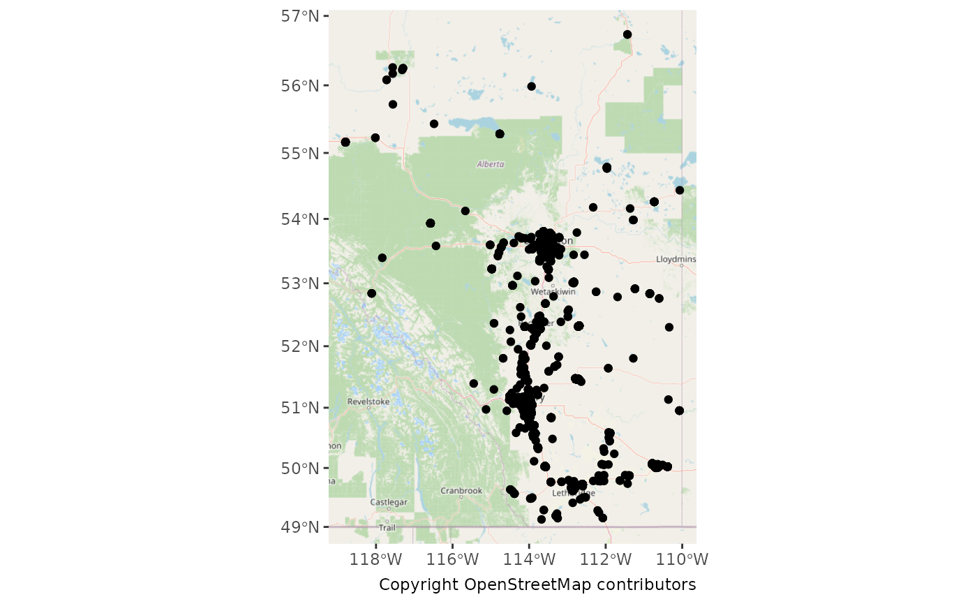
Let’s count our observations for each site.
cnt <- house_finches_sf |>
  count(geometry)

ggplot() +
  annotation_map_tile(type = "osm", zoomin = 0) +
  geom_sf(data = cnt, aes(size = n)) +
  labs(caption = "Copyright OpenStreetMap contributors")
## Zoom: 6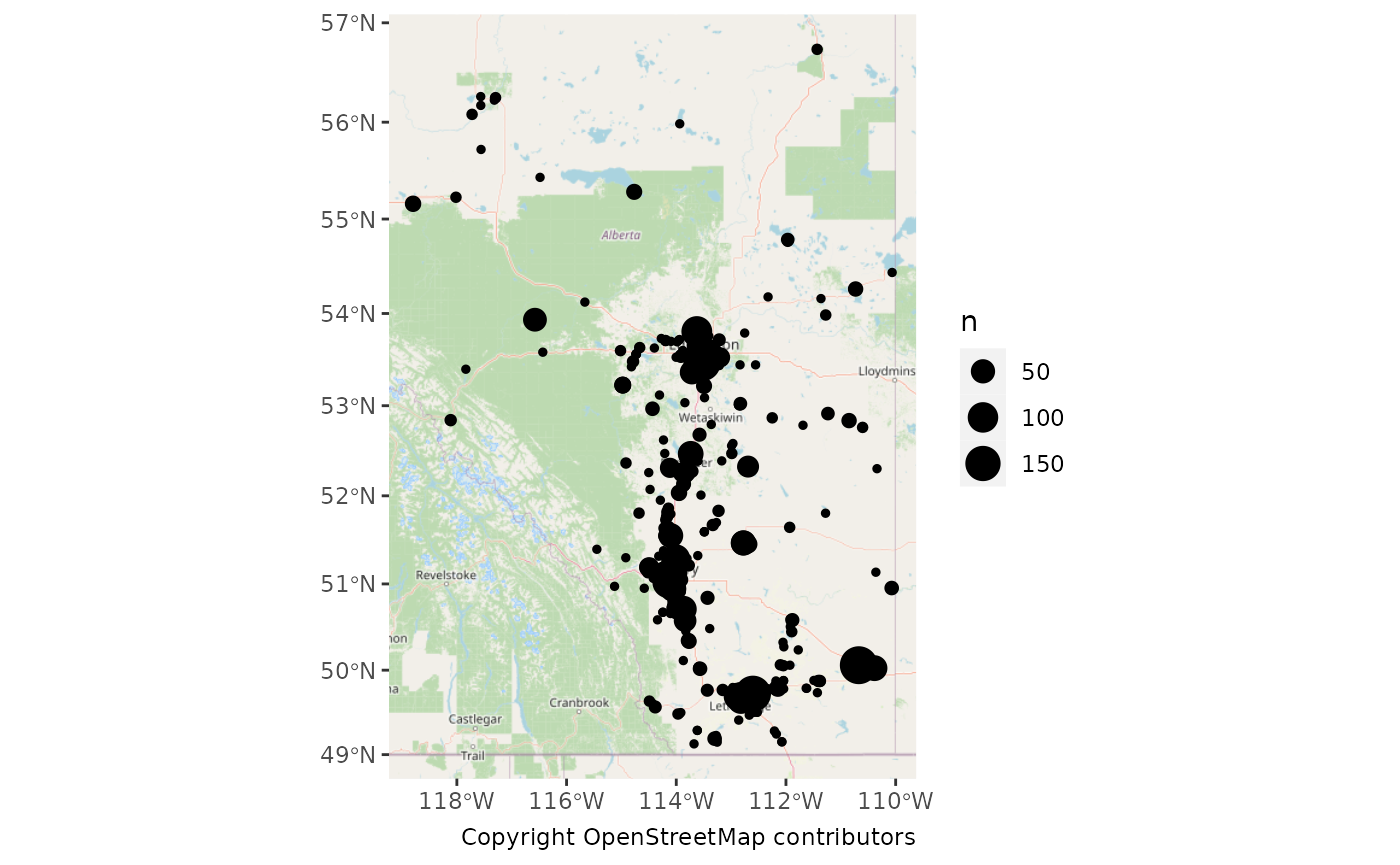
Interactive Maps
If we want to get fancy we can also create interactive maps using the
mapview packages (see also the leaflet for R
package).
More Complex Maps
For more complex, or detailed maps, we can use a variety of spatial data files to layer our data over maps of the area.
For this we’ll get some outlines of Canada and it’s Provinces and
Territories from rnaturalearth.
canada <- ne_states(country = "canada", returnclass = "sf") |>
  st_transform(3347)

ggplot() +
  theme_bw() +
  geom_sf(data = canada)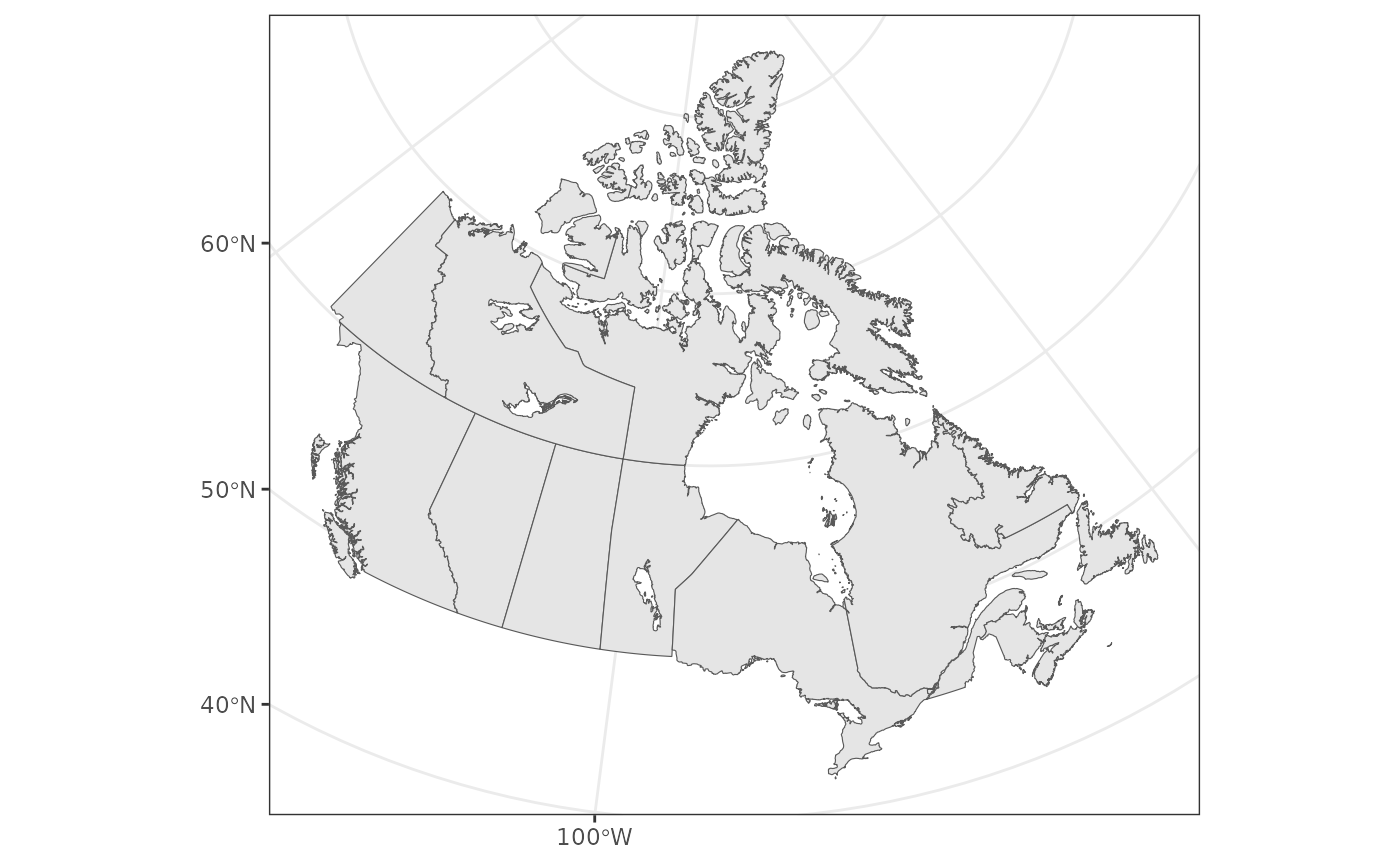
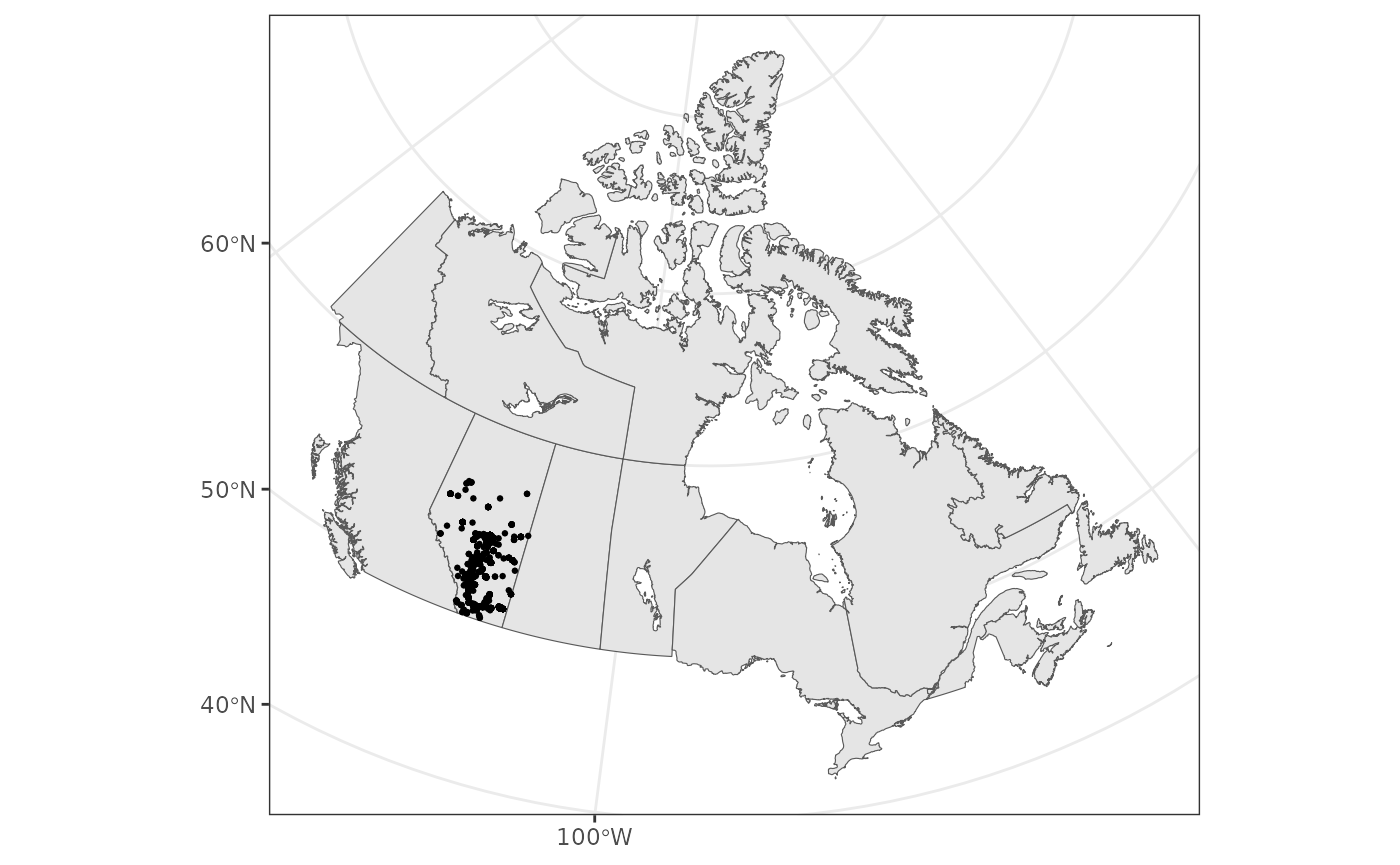
Let’s add our observations (note that the data are transformed to
match the projection of the first layer, here the canada
data).
We can also focus on Alberta
ab <- filter(canada, name == "Alberta")

ggplot() +
  theme_bw() +
  geom_sf(data = ab) +
  geom_sf(data = house_finches_sf, size = 0.5)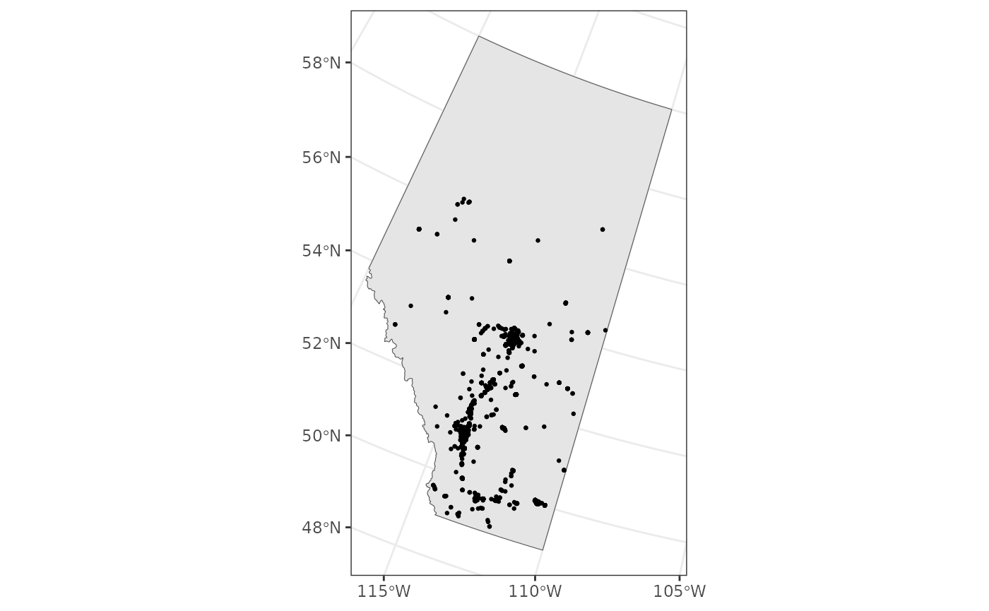
Perhaps we should see how these observations are distributed among Alberta’s Bird Conservation Regions (BCRs).
First we’ll grab the BCR shape file from Birds Canada1.
We’ll download the zip file and extracted to a folder easier to work
with. Note that these spatial data are in the GDB format, so we’re
working with a folder named XXX.gdb.
download.file(
  "https://services1.arcgis.com/d5M16PKlQTMEVyua/arcgis/rest/services/BCR_terrestrial_master/FeatureServer/replicafilescache/BCR_terrestrial_master_-8688020410858769740.zip",
  "BCR_terrestrial_master.zip"
)
unzip(
  "BCR_terrestrial_master.zip",
  junkpaths = TRUE,
  exdir = "BCR_terrestrial_master.gdb"
)
bcr <- st_read("BCR_terrestrial_master.gdb") |>
  st_transform(3347) |>
  st_intersection(ab)
## Reading layer `BCR_Terrestrial_Master' from data source
## `/home/runner/work/naturecounts/naturecounts/vignettes/articles/BCR_terrestrial_master.gdb'
## using driver `OpenFileGDB'## Warning in CPL_read_ogr(dsn, layer, query, as.character(options), quiet, : GDAL
## Message 1: organizePolygons() received a polygon with more than 100 parts. The
## processing may be really slow. You can skip the processing by setting
## METHOD=SKIP.## Simple feature collection with 4414 features and 8 fields
## Geometry type: MULTIPOLYGON
## Dimension: XY
## Bounding box: xmin: -6653676 ymin: -2736345 xmax: 2978061 ymax: 5253189
## Projected CRS: North_America_Lambert_Conformal_Conic## Warning: attribute variables are assumed to be spatially constant throughout
## all geometriesAdd this layer to our plot.
ggplot() +
  theme_bw() +
  geom_sf(data = ab) +
  geom_sf(data = bcr, aes(fill = factor(bcr_label)), alpha = 0.5, colour = NA) +
  geom_sf(data = house_finches_sf, size = 0.5) +
  scale_fill_viridis_d(name = "BCR")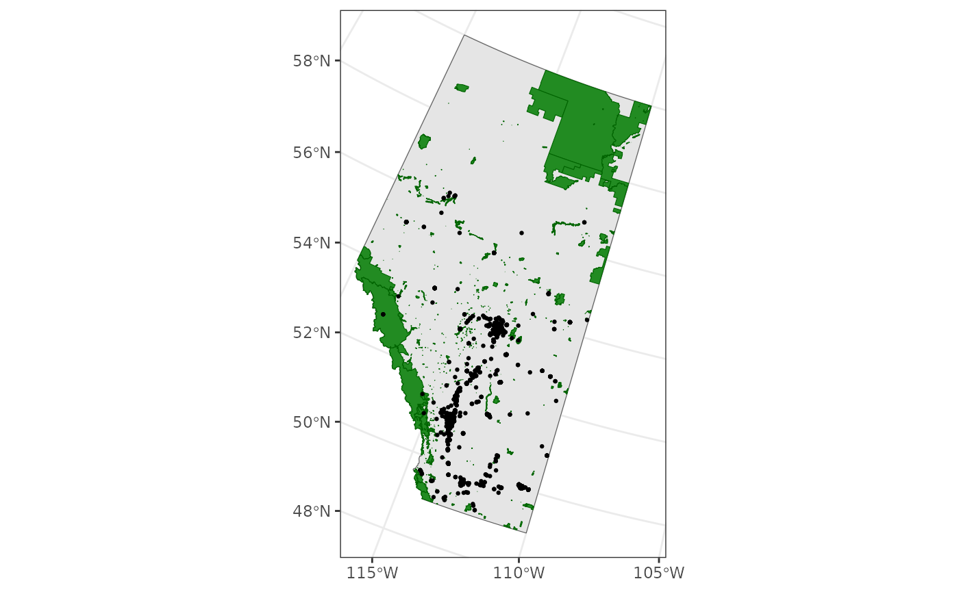
Some of the border cases are a bit hard to separate visually. To solve this problem, we can merge our observations with the BCRs and plot the observations by BCR as well.
First we’ll transform our observation data to match the CRS of
bcr, then we’ll join the BCR information to our
observations, based on whether the observations overlap a BCR polygon
(by default this is a left join). Now we have a BCR designation for each
observation.
house_finches_sf <- house_finches_sf |>
  st_transform(st_crs(bcr)) |>
  st_join(bcr)
Those border cases are now resolved.
ggplot() +
  theme_bw() +
  geom_sf(data = ab) +
  geom_sf(
    data = bcr,
    aes(fill = factor(bcr_label)),
    alpha = 0.25,
    colour = NA
  ) +
  geom_sf(data = house_finches_sf, aes(fill = factor(bcr_label)), shape = 21) +
  scale_fill_viridis_d(name = "BCR")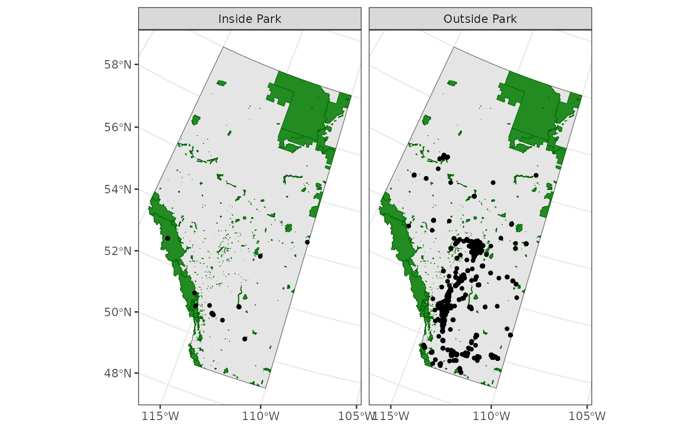
We might also be interested in observations over time.
First we’ll bin our yearly observations
house_finches_sf <- mutate(
  house_finches_sf,
  years = cut(
    survey_year,
    breaks = seq(1960, 2010, 10),
    labels = seq(1960, 2000, 10),
    right = FALSE
  )
)
We’ll also want to see how many sample years there are per decade.
years <- house_finches_sf |>
  group_by(years) |>
  summarize(n = length(unique(survey_year)), .groups = "drop")
Now we can see how House Finch observations change over the years
ggplot() +
  theme_bw() +
  geom_sf(data = ab) +
  geom_sf(data = bcr, aes(fill = factor(bcr_label)), alpha = 0.5, colour = NA) +
  geom_sf(data = house_finches_sf, size = 0.5) +
  scale_fill_viridis_d(name = "BCR") +
  geom_sf_text(
    data = years,
    x = 4427134,
    y = 2965275,
    hjust = 0,
    vjust = 1,
    aes(label = paste0("n = ", n))
  ) +
  facet_wrap(~years)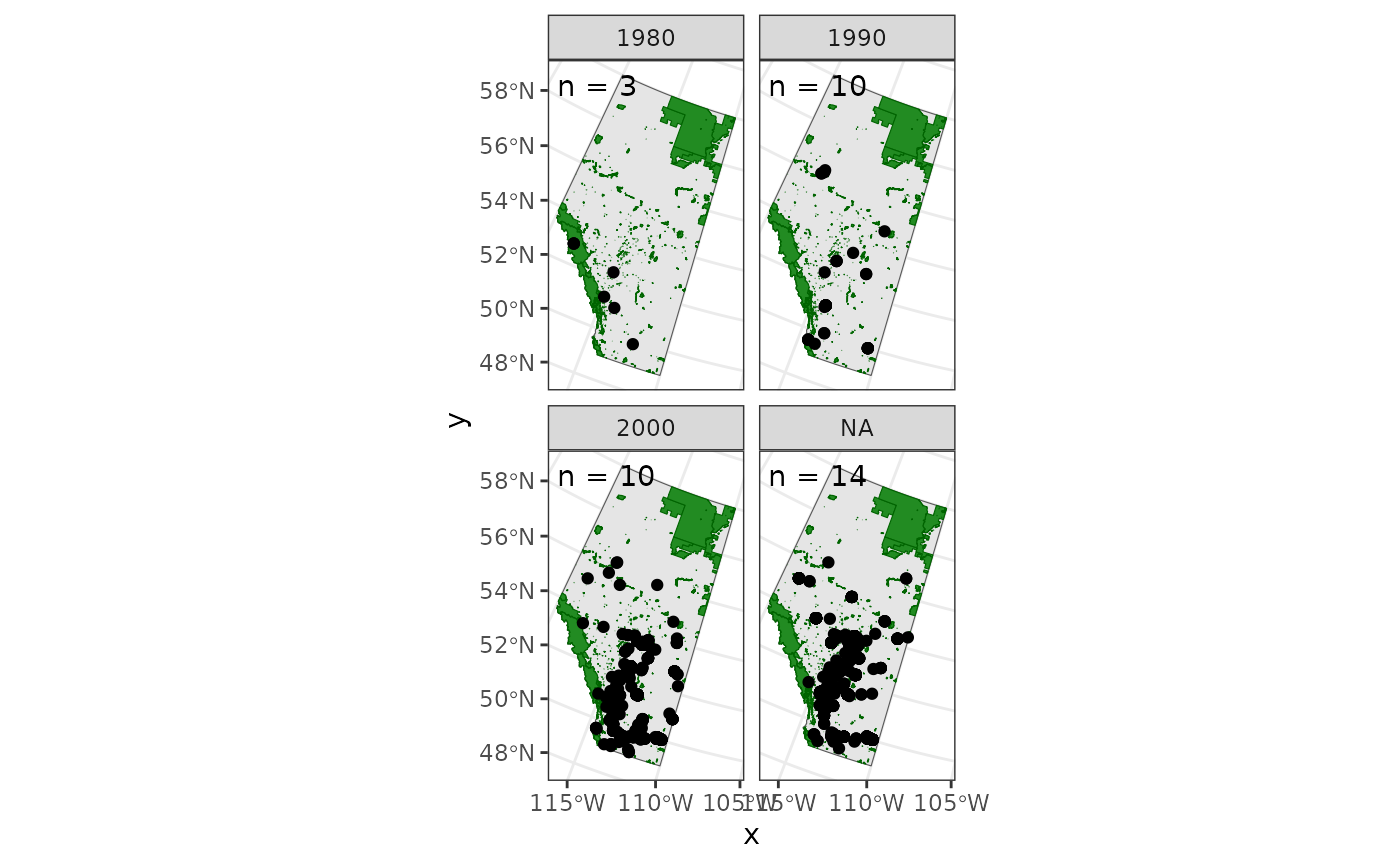
Presence/Absence
We can also use some of the naturecounts helper
functions to create presence/absence maps.
Here we download data from the RCBIOTABASE collection,
make sure to keep only observations where all species and the location
were reported, create a new presence column which is either
TRUE, FALSE, or NA for each sampling event. Finally we use the
format_zero_fill() function to fill in sampling events
where cardinals (species_id 19360) were not detected
(presence would then be 0).
cardinals <- nc_data_dl(
  collection = "RCBIOTABASE",
  username = "testuser",
  info = "nc_tutorial"
)
## Using filters: collections (RCBIOTABASE); fields_set (BMDE2.00-ext)## Collecting available records...## collection nrecords
## 1 RCBIOTABASE 13115
## Total records: 13,115##
## Downloading records for each collection:## RCBIOTABASE## Records 1 to 5000 / 13115## Records 5001 to 10000 / 13115## Records 10001 to 13115 / 13115
cardinals_zf <- cardinals |>
  filter(AllSpeciesReported == "Yes", !is.na(latitude), !is.na(longitude)) |>
  group_by(species_id, AllSpeciesReported, SamplingEventIdentifier) |>
  summarize(
    presence = sum(as.numeric(ObservationCount)) > 0,
    .groups = "drop"
  ) |>
  format_zero_fill(
    species = 19360,
    by = "SamplingEventIdentifier",
    fill = "presence"
  )
A bit convoluted, but here we’ll grab coordinates for each Sampling Event. This is only necessary if there are errors (worth reporting!) where there are more than one lat/lon combo for each sampling event.
coords <- cardinals |>
  select("SamplingEventIdentifier", "latitude", "longitude") |>
  group_by(SamplingEventIdentifier, latitude, longitude) |>
  mutate(n = n()) |> # Count number of unique coordinates
  group_by(SamplingEventIdentifier) |>
  slice_max(n, with_ties = FALSE) |> # Grab the most common coordinates for each event
  select(-"n")

cardinals_zf <- left_join(cardinals_zf, coords, by = "SamplingEventIdentifier")

head(cardinals_zf)
## SamplingEventIdentifier species_id presence latitude longitude
## 1 RCBIOTABASE-10000-1 19360 FALSE 45.58604 -77.48721
## 2 RCBIOTABASE-10001-1 19360 FALSE 45.51110 -77.50533
## 3 RCBIOTABASE-10002-1 19360 FALSE 45.50803 -77.50786
## 4 RCBIOTABASE-10003-1 19360 FALSE 45.51110 -77.50533
## 5 RCBIOTABASE-10004-1 19360 FALSE 45.51110 -77.50533
## 6 RCBIOTABASE-10005-1 19360 FALSE 45.51110 -77.50533Now that we have our presence/absence data for cardinals, we can create a map.
cnt <- st_as_sf(
  cardinals_zf,
  coords = c("longitude", "latitude"),
  crs = 4326
) |>
  group_by(presence) |>
  count(geometry)

ggplot() +
  annotation_map_tile(type = "osm", zoomin = 0) +
  geom_sf(data = cnt, aes(size = n, colour = factor(presence)), alpha = 0.5) +
  scale_colour_manual(
    name = "Presence/Absence",
    values = c("#31688E", "#440154"),
    labels = c("1" = "Present", "0" = "Absent")
  ) +
  scale_size_continuous(name = "Number of Sampling Events", range = c(1, 20)) +
  labs(
    caption = "Copyright OpenStreetMap contributors",
    title = "Presence/Absence of Cardinals in the RCBIOTABASE collection"
  )
## Zoom: 9## Fetching 16 missing tiles## | | | 0% | |==== | 6% | |========= | 12% | |============= | 19% | |================== | 25% | |====================== | 31% | |========================== | 38% | |=============================== | 44% | |=================================== | 50% | |======================================= | 56% | |============================================ | 62% | |================================================ | 69% | |==================================================== | 75% | |========================================================= | 81% | |============================================================= | 88% | |================================================================== | 94% | |======================================================================| 100%## ...complete!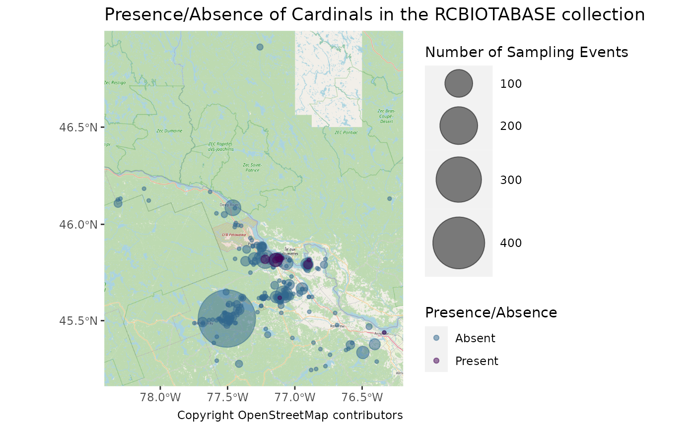
Clean up the mapping files if you no longer need them
unlink("alberta_parks/", recursive = TRUE)