Chapter 3 - Understanding and Viewing Data • naturecounts

Understanding and Viewing Data

This chapter begins with a brief introduction to the structure of the NatureCounts database, followed by a description of access levels and how to create a user account. We then provide instructions on how to view data from various collections and apply filters.

library(naturecounts)

The code in this Chapter will not work unless you replace "testuser" with your actual user name. You will be prompted to enter your password.

Data Structure

The Bird Monitoring Data Exchange (BMDE) was developed to be a standardized data exchange schema to promote the sharing and analysis of avian observational data. The schema is the core sharing standard of the Avian Knowledge Network.The BMDE (currently version 2.0) includes 169 core fields (variables) that are capable of capturing all metrics and descriptors associated with a bird observation. The BMDE schema was extended in 2018, and the complete version now includes 265 fields (variables).

Fields are variables or columns in a data set

By default, the naturecounts package downloads the data with the minimum set of fields/columns. However, for more advanced applications, users may wish to specify which fields/columns to return using the field_set and fields options in the nc_data_dl() function. For help with this feature, see the naturecounts article ‘Selecting columns and fields to download’.

Levels of Data Access

NatureCounts hosts many datasets, representing in excess of 170 million occurrence records, with a primary focus on Canadian bird monitoring data. Many of those datasets are from projects lead by Birds Canada and/or its partners. While we strive to make our data as openly available as possible, we also need to recognize the needs of our partners and funders.

NatureCounts has five Levels of Data Access, which define how each dataset can be used. Those levels are set individually for each dataset, in consultation with the various partners and data custodians involved.

Level 0: most restricted (archival only)
Level 1: archival only, metadata visible
Level 2: data used for visualizations only
Level 3: data available to third parties by request
Level 4: data shared with external portals and available by request
Level 5: open access

All contributing members of NatureCounts have complete authority over the use of the data they have provided, and can withhold data at any time from any party or application. All users of any NatureCounts data must clearly acknowledge the contribution of the members who are making data available. Each dataset comes with its own Data Sharing Policy that defines the various conditions for data usage.

You can view the Data Access Level for each collection on the NatureCounts Datasets page or using the metadata function (see akn_level):

collections<-meta_collections()
View(collections)

You can create a stand alone table for any metadata table using similar syntax as above

To retrieve the metadata for a specific set of collections based on its project_id, you can index the ‘collections’ dataframe.

# Specify the project_id you want to retrieve
projectID <- "insert_project_id_number"

# Subset to retrieve the relevant metadata based on project_id
collection_metadata <- collections[collections$project_id == projectID, ]

# View the metadata of the collection(s) with the specified project_id
if (nrow(collection_metadata) > 0) {
  View(collection_metadata)
} else {
  print("No collection found with the specified project_id.")
}

Authorizations

To access data using the naturecounts R package, you must sign up for a free account. Further, if you would like to access Level 3 or 4 collections you must make a data request. For step-by-step visual instructions, we encourage you to watch: NatureCounts: An Introductory Tutorial.

Create your free account now before continuing with this workbook

Viewing information about NatureCounts collections

First, lets use the naturecounts R package to view the number of records available for different collections. To do this we use the nc_count() function. You can view all the available collections and the number of observations using the default setting.

If a username is provided, the collections are filtered to only those available to the user. Otherwise all counts from all data sources are returned (default: show = "all").

nc_count <- nc_count()
View(nc_count)

Or you can view the collections for which you have access using your username/password.

nc_count <- nc_count(username = "testuser")
View(nc_count)

Further refinements can be applied to the nc_count() function using filters Options include: collections, project_id, species, years, doy (day-of-year), region, and site_type.

Metadata codes and descriptions

There are metadata associated with the various arguments used in the nc_count() and nc_data_dl() functions, the latter you will use in Chapter 4. These are stored locally and can be accessed anytime to help filter your data view or download query. They include:

meta_country_codes(): country codes
meta_statprov_codes(): state/Province codes
meta_subnational2_codes(): subnational2 codes
meta_iba_codes(): Important Bird Area (IBA) codes
meta_bcr_codes(): Bird Conservation Region (BCR) codes
meta_utm_squares(): UTM Square codes
meta_species_authority(): species taxonomic authorities
meta_species_codes(): alpha-numeric codes for avian species
meta_species_taxonomy(): codes and taxonomic information for all species
meta_collections(): collections names and descriptions
meta_breeding_codes(): breeding codes and descriptions
meta_project_protocols(): project protocols
meta_projects(): projects ids, names, websites, and descriptions
meta_protocol_types(): protocol types and descriptions

Any of these functions can be used to browse the code lists relevant to your search. For example, you can view the metadata for Birds Canada projects, including project ids using:

project_ids <- meta_projects() # retrieve the project_ids represented in the repository 
View(project_ids) # explore the dataframe

Using the above functions to search by country, state/province, subnational2, BCR etc. is especially useful for regional filtering in this next section.

Region & Species filtering

Filtering will often be done based on geographic extent (i.e., region). To filter by region you must provide a named list with one of the following:

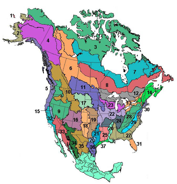
country: country code (e.g., CA for Canada)
statprov: state/province code (e.g., MB for Manitoba)
subnational2: subnational (type 2) code (e.g., CA.MB.07 for the Brandon Area)
iba: Important Bird Areas (IBA) code (e.g., AB001 for Beaverhill Lake in Alberta)
bcr: Bird Conservation Regions (e.g., 2 for Western Alaska)
utm_squares: UTM square code (e.g., 10UFE96 for a grid in Alberta)
bbox: bounding box coordinates (e.g., c(left = -101.097223, bottom = 50.494717, right = -99.511239, top = 51.027557) for a box containing Riding Mountain National Park in Manitoba). On the NatureCounts web portal there is a handy Within Coordinates) tool to help you retrieve custom coordinates for your data query and/or download.

The search_region function may be used to search a region by name (English or French) by specifying the ‘type’ argument.

For example, by country;

search_region("États-Unis", type = "country")

## # A tibble: 3 × 3
##   country_code country_name                         country_name_fr             
##   <chr>        <chr>                                <chr>                       
## 1 UM           United States Minor Outlying Islands Îles mineures éloignées des…
## 2 US           United States                        États-Unis                  
## 3 VI           Virgin Uslands, U.S.                 Îles Vierges des États-Unis

Or by Bird Conservation Region:

search_region("rainforest", type = "bcr")

## # A tibble: 1 × 4
##     bcr bcr_name                    bcr_name_es                      bcr_name_fr
##   <int> <chr>                       <chr>                            <chr>      
## 1     5 Northern Pacific Rainforest Bosque Lluvioso del Pacífico No… Forêts plu…

When using the nc_count() view function, you have the helpful option of filtering data by region. Let’s demonstrate how to use this function and the region argument with a few examples.

First, let’s limit our data search to Quebec:

nc_count(region = list(statprov="QC")) # filter nc_count by statprov

Next, let’s say we want to narrow down our search to the subnational level (Montreal and Toronto) but don’t know the corresponding codes for these regions.

Browse the code list:

View(meta_subnational2_codes())

Or, more efficiently, search by region:

search_region("Montreal", type = "subnational2")

## # A tibble: 1 × 5
##   country_code statprov_code subnational2_code subnational2_name      ebird_code
##   <chr>        <chr>         <chr>             <chr>                  <chr>     
## 1 CA           QC            CA.QC.MR          Communauté-Urbaine-de… CA-QC-MR

Great, we now know the codes we need and can view our metadata using nc_count():

nc_count(region = list(subnational2 = c("CA-QC-MR", "CA-ON-TO")))

## Without a username, using 'show = "all"'

## Using filters: subnational2 (CA-QC-MR, CA-ON-TO)

## # A tibble: 469 × 4
##    collection akn_level access     nrecords
##    <chr>          <int> <chr>         <int>
##  1 ABATLAS1           5 full         123364
##  2 ABATLAS2           5 full         201357
##  3 ABBIRDRECS         5 full         357264
##  4 ABOWLS             4 by request    20956
##  5 ACCWS              3 by request    22889
##  6 ATBANS             3 by request      267
##  7 ATOWLS             4 by request    34149
##  8 AWSGS              3 by request     8931
##  9 BBS                5 full        5735895
## 10 BBS50-CAN          5 full        4543180
## # ℹ 459 more rows

Similarly, this function can be used to view metadata for a bounding box using latitude and longitude coordinates:

nc_count(region = list(bbox = c(left = -125, bottom = 45, 
                                right = -100, top = 50)))

## Without a username, using 'show = "all"'

## Using filters: bbox_left (-125); bbox_bottom (45); bbox_right (-100); bbox_top (50)

## # A tibble: 169 × 4
##    collection      akn_level access     nrecords
##    <chr>               <int> <chr>         <int>
##  1 ABATLAS1                5 full           9827
##  2 ABATLAS2                5 full          25648
##  3 ABBIRDRECS              5 full          39546
##  4 ABOWLS                  4 by request      306
##  5 BBS                     5 full         373698
##  6 BBS50-CAN               5 full         414770
##  7 BBS50-US-WEST           5 full        1435081
##  8 BCATLAS1BE_DO           5 full           8786
##  9 BCATLAS1BE_RAW          5 full         106886
## 10 BCATLAS1BE_SUMM         5 full          41747
## # ℹ 159 more rows

Another commonly used filter is specific to species. In order to filter by species you need to get the species id codes. These are numeric codes that reflect species identity.

For all species, you can search the NatureCounts repository by scientific, English or French name with the search_species() function.

search_species("chickadee") # returns all chickadee species ids

The corresponding species id can then be used to download the data either directly or by saving and referencing the data frame: see Chapter 4

For birds, you can also search by alphanumeric species code with the search_species_code() function.

species_codes <- search_species_code() # returns all species codes represented in the database.

This function, by default, uses the BSCDATA taxonomic authority and returns all species codes related to the search term including related subspecies. For this reason, it is considered a more robust method for ensuring that you do not miss observations in your search.

If you’re interested in a particular species, and any recognized subspecies, you can filter your search:

search_species_code("BCCH") # Filters by species code

The search function is case insensitive:

search_species_code("bcch") # Also filters by species code

## # A tibble: 1 × 5
##   species_id BSCDATA scientific_name      english_name           french_name    
##        <int> <chr>   <chr>                <chr>                  <chr>          
## 1      14280 BCCH    Poecile atricapillus Black-capped Chickadee Mésange à tête…

It is important to note that species subdivisions (subspecies, subpopulations, hybrids, etc.) can also be recognized with different codes across taxonomic authority (BSCDATA, CBC).

For example, BSCDATA recognizes 3 sub groups of the Dark-eyed junco:

search_species_code("DEJU") # Returns species ids for Junco hyemali and 3 related subgroups

## # A tibble: 4 × 5
##   species_id BSCDATA scientific_name                    english_name french_name
##        <int> <chr>   <chr>                              <chr>        <chr>      
## 1      19090 SCJU    Junco hyemalis hyemalis/carolinen… Dark-eyed J… Junco ardo…
## 2      19110 PSJU    Junco hyemalis mearnsi             Dark-eyed J… Junco ardo…
## 3      42218 DEJU    Junco hyemalis                     Dark-eyed J… Junco ardo…
## 4      47928 ORJU    Junco hyemalis [oreganus Group]    Dark-eyed J… Junco ardo…

We have to modify our search when filtering by the CBC code system. This taxonomic authority recognizes 9 sub group hybrids of the Dark-eyed junco, as well as the Guadalupe junco:

search_species_code("12385", authority = "CBC") # Returns the species ids and CBC codes for Junco hyemali, 9 subgroups, and the Guadelupe junco

## # A tibble: 11 × 5
##    species_id CBC   scientific_name                     english_name french_name
##         <int> <chr> <chr>                               <chr>        <chr>      
##  1      42218 12385 Junco hyemalis                      Dark-eyed J… Junco ardo…
##  2      19090 12386 Junco hyemalis hyemalis/carolinens… Dark-eyed J… Junco ardo…
##  3      41434 12388 Junco hyemalis cismontanus          Dark-eyed J… Junco ardo…
##  4      19100 12389 Junco hyemalis [oreganus Group]     Dark-eyed J… Junco ardo…
##  5      19110 12390 Junco hyemalis mearnsi              Dark-eyed J… Junco ardo…
##  6      42219 12391 Junco hyemalis [oreganus Group] x … Dark-eyed J… Junco ardo…
##  7      19112 12392 Junco hyemalis aikeni               Dark-eyed J… Junco ardo…
##  8      19111 12394 Junco hyemalis caniceps             Dark-eyed J… Junco ardo…
##  9      42220 12395 Junco hyemalis mearnsi x caniceps   Dark-eyed J… Junco ardo…
## 10      40859 12396 Junco hyemalis dorsalis             Dark-eyed J… Junco ardo…
## 11      39768 12398 Junco insularis                     Guadalupe J… Junco de G…

You can search by more than one authority at the same time. Note that your search term only needs to match one authority (not both), and that the information returned reflects both authorities combined.

View(search_species_code("DEJU", authority = c("BSCDATA", "CBC")))

If you do not want all subgroups, you can use the results = “exact” argument to return only an exact match.

search_species_code("DEJU", results = "exact")

## # A tibble: 1 × 5
##   species_id BSCDATA scientific_name english_name    french_name  
##        <int> <chr>   <chr>           <chr>           <chr>        
## 1      42218 DEJU    Junco hyemalis  Dark-eyed Junco Junco ardoisé

For additional examples and more advanced options are available online for retrieving Region and Species codes.

Examples

Here are a few examples for you to work through to become familiar with the nc_count() function.

Example 1: Determine the number of collections and records for a specific region. The options include: country, statprov, subnational2, iba, bcr, utm_squares, and bbox. You can find details and examples on how to search_region() at the link provided.

The following code will retrieve all available collections and number of records for British Columbia

search_region("British Columbia", type = "statprov")
nc_count(region = list(statprov = "BC"))

Example 2: Determine the number of records for a specific species. You can find details and examples on how to search_species_code() based on 4 letter alpha code and search_species() based on common names at the links provided.

The following code will retrieve all available collections and number of records for Red-headed Woodpecker

search_species("Red-headed Woodpecker")
search_species_code("RHWO")

RHWO<-nc_count(species = 10060)
View(RHWO)

Example 3: We can further refine the Red-headed Woodpecker example (above) by filtering the species-specific data by region (e.g., Bird Conservation Region 11), time period (e.g., 2015-2019), or a combination of both.

RHWO_11 <- nc_count(species = 10060, region = list(bcr = "11"))
View(RHWO_11)

RHWO_year <- nc_count(species = 10060, year = c(2015, 2019))
View(RHWO_year)

RHWO_11_year <- nc_count(species = 10060, region = list(bcr = "11"), year = c(2015, 2019))
View(RHWO_11_year)

Exercises

Now apply your newly acquired skills!

Exercise 1: If you are interesting in doing a research project on Snowy Owls in Quebec, which three collections are you most likely to consider using (i.e., which have the most data)?

Answer: EBird-CA-QC, OISEAUXQC, CBC

Exercise 2: How many records of Gadwal are in the British Columbia Coastal Waterbird Survey collection? What if you are only interested in records from 2010-2019, how many records are available?

Answer: 702, 389

Full answers to the exercises can be found in Chapter 7.

Chapter 3 - Understanding and Viewing Data

2025-04-07