In this section we’ll explore Important Bird Areas (IBAs) and Bird Conservation Regions (BCRs), so you’ll have a better idea of what they represent when used as data filters.
We’ll be using the tidyverse packages
dplyr and ggplot2 for data manipulation and
plotting, respectively. We’ll use the sf package for
working with spatial data, and the rnaturalearth package to
get example spatial data.
library(naturecounts)
library(dplyr)
library(ggplot2)
library(sf)
library(rnaturalearth)
library(mapview)First we’ll get some spatial objects for our explorations from the
rnaturalearth package. A map of North America and of
Canada, both transformed from CRS EPSG code 4326 (unprojected lat/lon)
to 3347 (NAD83 Statistics Canada).
na <- ne_countries(continent = "north america", returnclass = "sf") |>
st_transform(3347)
canada <- ne_states(country = "canada", returnclass = "sf") |>
st_transform(3347)Important Bird Areas
To get a visual idea of where different Important Bird Areas are, let’s plot them on our map of Canada.
First we need to grab the IBA data frame and convert it to a spatial object. Because the data contains lat/lon, we assign it to CRS 4326 for GPS lat/lon data, and then convert it to match the crs of our maps.
iba <- meta_iba_codes() |>
st_as_sf(coords = c("longitude", "latitude"), crs = 4326) |>
st_transform(3347)
ggplot() +
theme_bw() +
geom_sf(data = canada) +
geom_sf(data = iba)
If you want to narrow in on only one province,
- filter the IBA data frame
iba_nwt <- filter(iba, statprov == "NT")- get the limits of the Northwest Territories
Put it all together
ggplot() +
theme_bw() +
geom_sf(data = canada) +
geom_sf(data = iba_nwt) +
geom_sf_text(data = iba_nwt, aes(label = iba_site), size = 3, vjust = -0.5) +
coord_sf(xlim = limits[c("xmin", "xmax")], ylim = limits[c("ymin", "ymax")])
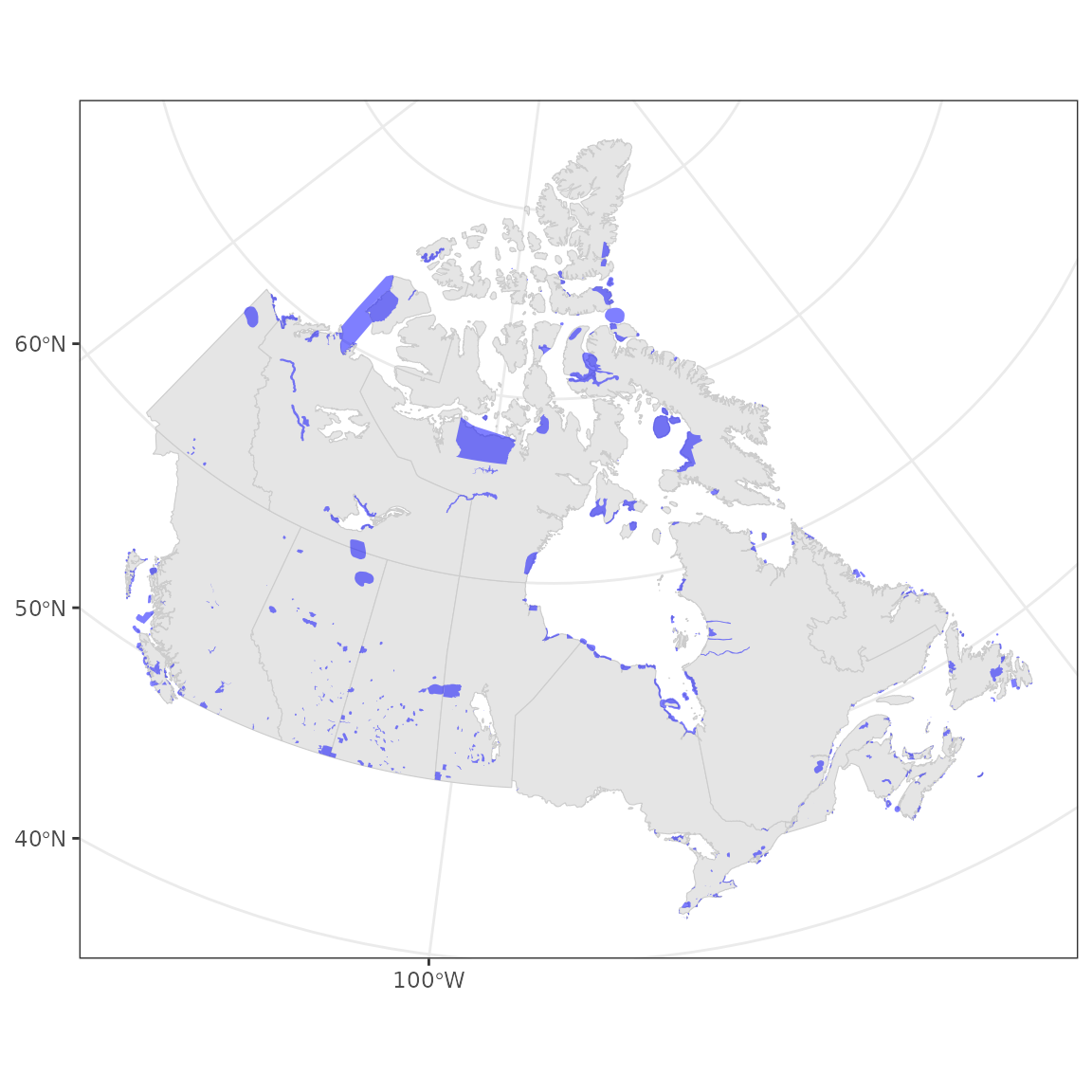
For a more detailed view of IBAs, we can also grab the shape files from Birds Canada.
iba <- st_read("https://birdmap.birdscanada.org/geoserver/atlas/ows?service=WFS&version=1.0.0&request=GetFeature&typeName=atlas:iba&outputFormat=application%2Fjson") |>
st_transform(3347)## Reading layer `OGRGeoJSON' from data source
## `https://birdmap.birdscanada.org/geoserver/atlas/ows?service=WFS&version=1.0.0&request=GetFeature&typeName=atlas:iba&outputFormat=application%2Fjson'
## using driver `GeoJSON'
## Simple feature collection with 619 features and 7 fields
## Geometry type: MULTIPOLYGON
## Dimension: XY
## Bounding box: xmin: -141.2376 ymin: 41.67177 xmax: -52.66698 ymax: 78.10591
## Geodetic CRS: WGS 84
iba <- filter(iba, Status == "confirmed") # Omit historical areas
ggplot() +
theme_bw() +
geom_sf(data = canada, colour = "grey80") +
geom_sf(data = iba, fill = "blue", colour = NA, show.legend = FALSE, alpha = 0.5)
To really explore these areas, interactive maps can be really useful. Note that you can move the map, zoom in and out, and click on specific IBAs for more information.
mapview(iba)Bird Conservation Regions
Bird Conservation Regions are also available from Birds Canada.
bcr <- st_read("https://birdmap.birdscanada.org/geoserver/atlas/ows?service=WFS&version=1.0.0&request=GetFeature&typeName=atlas:bcr&outputFormat=application%2Fjson") |>
st_transform(3347)## Reading layer `OGRGeoJSON' from data source
## `https://birdmap.birdscanada.org/geoserver/atlas/ows?service=WFS&version=1.0.0&request=GetFeature&typeName=atlas:bcr&outputFormat=application%2Fjson'
## using driver `GeoJSON'
## Simple feature collection with 66 features and 3 fields
## Geometry type: MULTIPOLYGON
## Dimension: XY
## Bounding box: xmin: -179.1335 ymin: 14.54426 xmax: -52.54375 ymax: 83.14808
## Geodetic CRS: WGS 84
ggplot() +
theme_bw() +
geom_sf(data = na, colour = "grey80") +
geom_sf(data = bcr, aes(fill = bcr), show.legend = FALSE, alpha = 0.5) +
scale_fill_viridis_c()
And again, interactive maps can be really useful.
mapview(bcr)