The COSEWIC Index of Area of Occupancy (IAO; also called Area of Occupancy, AOO by the IUCN) and Extent of Occurrence (EOO; IUCN as well) are metrics used to support status assessments for potentially endangered species.
Usage
cosewic_ranges(
  df_db,
  record = "record_id",
  coord_lon = "longitude",
  coord_lat = "latitude",
  group = "species_id",
  prop_include = 1,
  iao_grid_size_km = 2,
  iao_grid = NULL,
  eoo_clip = NULL,
  crs = "ESRI:102001",
  which = c("eoo", "iao"),
  filter_unique = FALSE,
  spatial = TRUE,
  species,
  eoo_p
)
Arguments
- df_db
Either data frame or a connection to database with
naturecountstable.- record
Character. Name of the column containing record identification.
- coord_lon
Character. Name of the column containing longitude.
- coord_lat
Character. Name of the column containing latitude.
- group
Character. Name of the column containing group identification. By default this is
species_idin NatureCounts data.- prop_include
Numeric. The proportion of points to include in the range calculations (applies to both IAO and EOO calculations). This proportion of points closest to the centroid of the data are retained. Defaults to 1 for 100% of points. Note that you may wish to use 0.95 to omit potential outlier points.
- iao_grid_size_km
Numeric. Size of grid (km) to use when calculating IAO. Default is COSEWIC requirement (2km, meaning 2x2km grids of 4km2). Use caution if changing.
- iao_grid
sf Polygon. Supply your own IAO grid rather than creating one. The CRS of this grid must be the same as
crs.- eoo_clip
sf (Multi)Polygon. A spatial object to clip the EOO to. May be relevant when calculating EOOs for complex regions (i.e. long curved areas) to avoid including area which cannot have observations.
- crs
A coordinate reference system (see
?sf::st_transform()). Defaults to Albers Equal-Area for Canada (ESRI:102001) for area calculations. Note that it must be a projection (i.e. not simply a reference system like 4326 used for GPS) for area calculations. IfNULLfor plots, uses the CRS of the base map or of the IAO/EOO data.- which
Character vector. Which range types to calculate. Any combination of "eoo" and "iao", default is both.
- filter_unique
Logical. Whether to filter observations to unique locations. Use this only if there are too many data points to work with. This changes the nature of what an observation is, and may also affect which observations are omitted if using
prop_include < 1.- spatial
Logical. Whether to return sf spatial objects showing calculations. If
TRUE(default) returns a list spatial data frames,iaoandeoo. IfFALSEreturns a data frame with IAO and EOO values.- species
Deprecated. Use
groups.- eoo_p
Deprectated. User
prop_include.
Value
If spatial = TRUE, a list with two spatial data frames, iao and
eoo. Otherwise a data frame.
(Spatial) data frames contain the following columns
Group column (defined by
group, defaults tospecies_id)n_records_total- Total number of records used to create ranges (after filtering ifprop_include < 1)prop_include- The proportion of original points included in these calculations
Additionally the iao data frame contains
grid_id- ID number for grid cellsn_records- Number of records in that grid cellmin_record- Minimum number of records across all cellsmax_record- Maximum number of records across all cellsmedian_record- Median number of records across all cellsgrid_size_km- IAO cell size in km (i.e. width)n_occupied- Across all cells, number of IAO cells with at least one recordiao- IAO value (grid_size_km^2 *n_occupied)
Additionally the eoo data frame contains
eoo- EOO area calculated from the Convex Hull
Details
Note that the while the IUCN calls this metric AOO, in COSEWIC, AOO is actually a different measure, the biological area of occupancy. See the "Distribution" section in 'Instructions for preparing COSEWIC status reports' for more details.
By default ranges are calculated using all points (prop_include = 1)
However, if you're working on rough data or want to do a rough first pass,
you may wish to use prop_include = 0.95 to include only 95% of points
(based on distance to the centroid). This will ensure outlier observations
will not artificially inflate the EOO. Although the IAO is less sensitive to
outliers, to maintain consistency in the data the same observations are used
in both range calculations.
For a final COSEWIC assessment report, however, it is likely better to
carefully explore the data to ensure there are no outliers and then use the
full data set (i.e. use the default of prop_include = 1).
The IAO is calculated by first assessing large grids (10x large than the specified size). Only then are smaller grids created within large grid cells containing observations. This speeds up the process by avoiding the creation of grids in areas where there are no observations. This means that the plots and spatial objects may not have grids over large areas lacking observations. See examples.
Details on how IAO and EOO are calculated and used
Examples
# Using the included, test data on black-capped chickadees
r <- cosewic_ranges(bcch)
r
#> $iao
#> Simple feature collection with 475 features and 11 fields
#> Geometry type: POLYGON
#> Dimension: XY
#> Bounding box: xmin: 1407460 ymin: 785222 xmax: 1537823 ymax: 867036.6
#> Projected CRS: Canada_Albers_Equal_Area_Conic
#> # A tibble: 475 × 12
#> species_id n_records_total grid_id n_records min_record max_record
#> <int> <int> <int> <int> <int> <int>
#> 1 14280 160 1 0 1 35
#> 2 14280 160 2 0 1 35
#> 3 14280 160 3 0 1 35
#> 4 14280 160 4 0 1 35
#> 5 14280 160 5 0 1 35
#> 6 14280 160 6 0 1 35
#> 7 14280 160 7 0 1 35
#> 8 14280 160 8 0 1 35
#> 9 14280 160 9 0 1 35
#> 10 14280 160 10 0 1 35
#> # ℹ 465 more rows
#> # ℹ 6 more variables: median_record <int>, grid_size_km [km], n_occupied <int>,
#> # iao [km^2], prop_include <dbl>, geometry <POLYGON [m]>
#>
#> $eoo
#> Simple feature collection with 1 feature and 4 fields
#> Geometry type: POLYGON
#> Dimension: XY
#> Bounding box: xmin: 1415235 ymin: 792053.4 xmax: 1535250 ymax: 866555.2
#> Projected CRS: Canada_Albers_Equal_Area_Conic
#> # A tibble: 1 × 5
#> species_id n_records_total eoo prop_include x
#> <int> <int> [km^2] <dbl> <POLYGON [m]>
#> 1 14280 160 4729. 1 ((1426543 792053.4, 1415235 86…
#>
r <- cosewic_ranges(bcch, spatial = FALSE)
r
#> # A tibble: 1 × 10
#> species_id n_records_total min_record max_record median_record grid_size_km
#> <int> <int> <int> <int> <int> [km]
#> 1 14280 160 1 35 1 2
#> # ℹ 4 more variables: n_occupied <int>, iao [km^2], eoo [km^2],
#> # prop_include <dbl>
# Calculate for multiple groups
mult <- rbind(bcch, hofi)
r <- cosewic_ranges(mult)
r <- cosewic_ranges(mult, spatial = FALSE)
# Consider the Ontario MNR Lambert projection (all observations are in Ontario)
r2 <- cosewic_ranges(mult, crs = 3162)
# Clip to a specific region
library(rnaturalearth)
ON <- ne_states("Canada") %>%
dplyr::filter(postal == "ON")
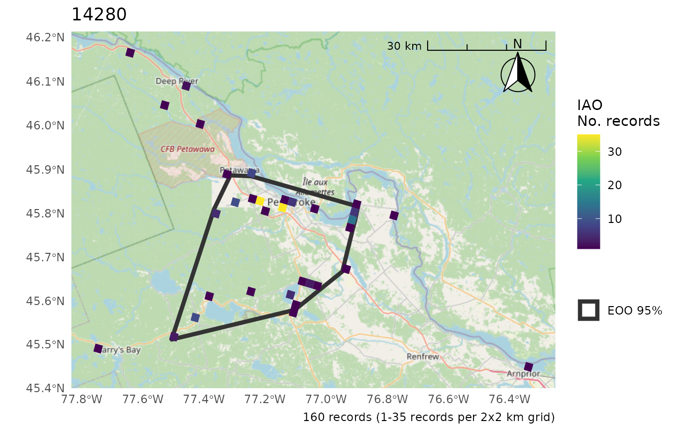
r <- cosewic_ranges(mult)
cosewic_plot(r, map = ON) # No clip
#> $`14280`
#> Scale on map varies by more than 10%, scale bar may be inaccurate
 #>
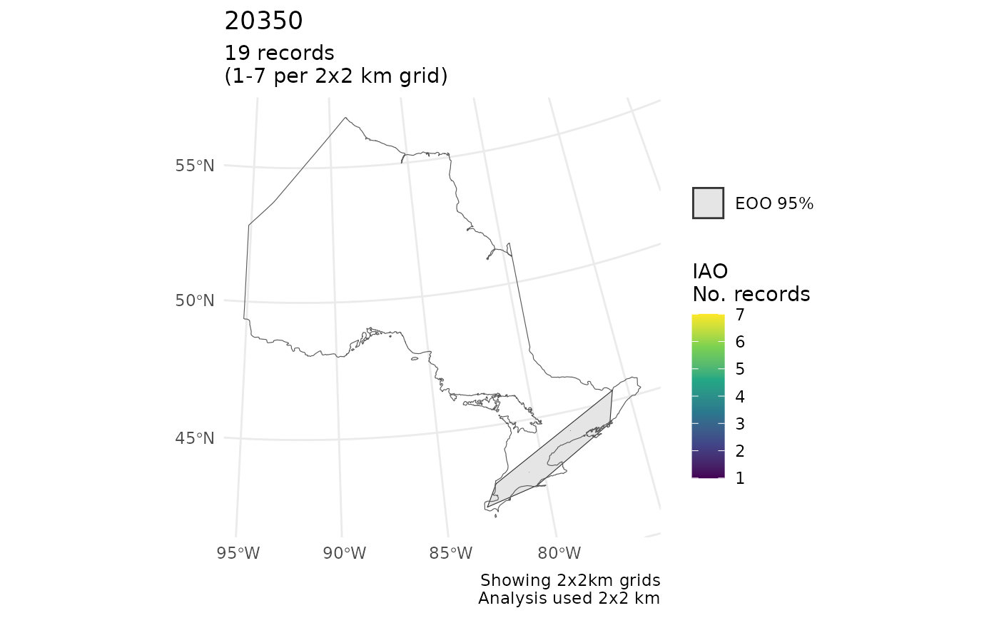
#> $`20350`
#> Scale on map varies by more than 10%, scale bar may be inaccurate
#>
#> $`20350`
#> Scale on map varies by more than 10%, scale bar may be inaccurate
 #>
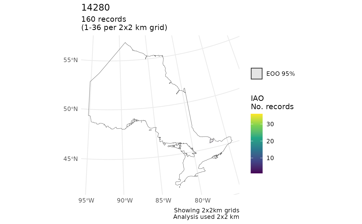
r <- cosewic_ranges(mult, eoo_clip = ON)
cosewic_plot(r, map = ON) # With clip
#> $`14280`
#> Scale on map varies by more than 10%, scale bar may be inaccurate
#>
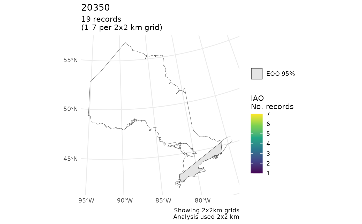
r <- cosewic_ranges(mult, eoo_clip = ON)
cosewic_plot(r, map = ON) # With clip
#> $`14280`
#> Scale on map varies by more than 10%, scale bar may be inaccurate
 #>
#> $`20350`
#> Scale on map varies by more than 10%, scale bar may be inaccurate
#>
#> $`20350`
#> Scale on map varies by more than 10%, scale bar may be inaccurate
 #>
# Use a custom IAO grid
# Load the demo grid for the bcch data set
grid <- sf::st_read(system.file(
"extdata",
"iao_bcch_grid.gpkg",
package = "naturecounts"
))
#> Reading layer `iao_bcch_grid' from data source
#> `/home/runner/work/_temp/Library/naturecounts/extdata/iao_bcch_grid.gpkg'
#> using driver `GPKG'
#> Simple feature collection with 3575 features and 1 field
#> Geometry type: POLYGON
#> Dimension: XY
#> Bounding box: xmin: 1406468 ymin: 786875.6 xmax: 1535250 ymax: 894738.5
#> Projected CRS: Canada_Albers_Equal_Area_Conic
r <- cosewic_ranges(bcch, iao_grid = grid)
#> User-provided grid has cell size of 2 [km]
cosewic_plot(r)
#> Zoom: 9
#>
# Use a custom IAO grid
# Load the demo grid for the bcch data set
grid <- sf::st_read(system.file(
"extdata",
"iao_bcch_grid.gpkg",
package = "naturecounts"
))
#> Reading layer `iao_bcch_grid' from data source
#> `/home/runner/work/_temp/Library/naturecounts/extdata/iao_bcch_grid.gpkg'
#> using driver `GPKG'
#> Simple feature collection with 3575 features and 1 field
#> Geometry type: POLYGON
#> Dimension: XY
#> Bounding box: xmin: 1406468 ymin: 786875.6 xmax: 1535250 ymax: 894738.5
#> Projected CRS: Canada_Albers_Equal_Area_Conic
r <- cosewic_ranges(bcch, iao_grid = grid)
#> User-provided grid has cell size of 2 [km]
cosewic_plot(r)
#> Zoom: 9
 # Slight differences when compared to internally created grid,
# just due to where the observations line up
r <- cosewic_ranges(bcch)
cosewic_plot(r)
#> Zoom: 9
# Slight differences when compared to internally created grid,
# just due to where the observations line up
r <- cosewic_ranges(bcch)
cosewic_plot(r)
#> Zoom: 9