Chapter 2 - Auxiliary Tables • naturecounts

Chapter 2: Auxiliary Tables from NatureCounts

In Chapter 1: Zero-filling, you explored three different methods that can be used to zero-fill NatureCounts data and generate presence/absence records. In this tutorial, you will explore custom table queries and create basic data summaries and maps using the rNest auxiliary table.

2.0 Learning Objectives

By the end of Chapter 2 - Auxiliary Tables, users will know how to:

Access NatureCounts auxiliary tables: Access Auxiliary Tables
Filter and view NatureCounts auxiliary tables: Filter Auxiliary Tables
Convert Julian dates to month, day, and time: rNest - Initiation and Fledging Dates
Combine spatial data by attribute field: rNest - Ecodistricts
Create basic data summaries: rNest - Data Summary
Map rNest data across ecodistricts: rNest - Mapping

This R tutorial requires the following packages:

library(naturecounts)
library(tidyverse)
library(lubridate)
library(sf)

2.1 Accessing Auxiliary Tables From `naturecounts`

NatureCounts hosts a variety of useful datasets that exist outside of the bird monitoring projects available for download online or through the nc_data_dl() function in R.

To browse the list of available auxiliary data tables, we can use the nc_query_table() function. Specify your naturecounts username for the complete list based on your access level. You will be prompted to enter your password.

nc_query_table(username = "testuser")
#>              table_name                        filters required
#> 1    AtlasSquareSummary                 statprove_code       NA
#> 2 bmde_filter_bad_dates project_id,SiteCode,species_id       NA
#> 3                 Rnest                           <NA>       NA
#> 4    SpeciesLifeHistory                           <NA>       NA

You’ll notice the filters and required columns. The former refers to the unique filter arguments that may be used for each table in your download queries. what does the required column signify?

To download a specific table like Rnest from the list, specify the table argument.

rnest <- nc_query_table(table = "Rnest", username = "testuser")

2.2 Filtering Auxiliary Tables From `naturecounts`

Built-in filters can be useful to query specific datasets.

For example, you can query the AtlasSquareSummary table by statprov_code.

atlas_square_summ_on <- nc_query_table(table = "AtlasSquareSummary", username = "testuser",
                                       statprov_code = "ON") # filter data for Ontario

You can also query the bmde_filter_bad_dates table by project_id, SiteCode, or species_id.

bmde_fbd_query <- nc_query_table(table = "bmde_filter_bad_dates", username = "testuser", project_id = "1013")

You can otherwise query any table by any relevant column after download, like species_id.

rnest_query <- filter(rnest, speciesID %in% c(15770, 47674)) # filter for the American Robin and Common Gull

2.3 rNest: Initiation and Fledging Dates

rNest is an R package that enables the backcalculation of nest chronologies from nest observations. It helps describe nesting phenology based on nest records held in the BirdsCanada database. The development of this package aims to produce a robust description of bird nesting phenology for 311 bird species across Canada. See the report here.

Initiation date - estimated date when the first egg was laid for each nest attempt.

Fledging date - estimated date that the first nestling leaves the nest, for each nest attempt.

Let’s examine the rNest query we performed for the American Robin and Common Gull in the last step. The initiation and fledging dates use the Julian date format. We can convert these dates to the day, month, and time-of-day for each event, respectively.

Ensure that each column is in numeric format.

rnest_query <- rnest_query %>%
  mutate(across(c(initiation, fledging), as.numeric))

Create an arbitrary base date, assuming the event dates are not for a leap year.

base_date <- as.Date("2025-01-01")

Create two new date columns by converting the Julian dates to standard format.

rnest_query <- rnest_query %>%
  mutate(
    initiation_date = base_date + initiation - 1,
    fledging_date = base_date + fledging - 1
  )

Extract the fractional Julian dates and convert to time.

rnest_query <- rnest_query %>%
  mutate(
    initiation_time = hours(round((initiation - floor(initiation)) * 24)),
    fledging_time = hours(round((fledging - floor(fledging)) * 24))
  )

Extract month and day using the month() and day() functions from the lubridate package.

rnest_query <- rnest_query %>%
  mutate(
    initiation_month = month(initiation_date),
    initiation_day = day(initiation_date),
    fledging_month = month(fledging_date),
    fledging_day = day(fledging_date)
  ) %>%
  dplyr::select(
    speciesID,
    speciesEnglish,
    speciesFrench,
    initiation,
    initiation_month,
    initiation_day,
    initiation_time,
    fledging,
    fledging_month,
    fledging_day,
    fledging_time,
    districtID,
    districtNameEn
  )

2.4 rNest: Ecodistricts

To help represent the rNest data visually, we’ll incorporate spatial data from the The National Ecological Framework for Canada which is available here. For more in-depth examples on manipulating NatureCounts and spatial data, see the NatureCounts_SpatialData_Tutorial series.

The rNest data contains the districtID field, which refers to the ecodistrict where the observation event took place. An ecodistrict is a subdivision of an ecoregion and is characterized by distinctive assemblages of relief, landforms, geology, soil, vegetation, water bodies and fauna.

The Ecodistricts spatial data is available as a series of pre-packaged GeoJSON files in this subdirectory. Were interested in the base layer GeoJSON file, displayed in raw text format at this URL.

Read in the Ecodistricts layer from the URL using the st_read() function.

# Copy-paste the URL to the Ecodistricts base-layer
geojson_url <- "https://agriculture.canada.ca/atlas/data_donnees/nationalEcologicalFramework/data_donnees/geoJSON/ed/nef_ca_ter_ecodistrict_v2_2.geojson"

# Read the GeoJSON file directly from the URL
ecodistricts <- st_read(geojson_url)
#> Reading layer `nef_ca_ter_ecodistrict_v2_2' from data source 
#>   `https://agriculture.canada.ca/atlas/data_donnees/nationalEcologicalFramework/data_donnees/geoJSON/ed/nef_ca_ter_ecodistrict_v2_2.geojson' 
#>   using driver `GeoJSON'
#> Simple feature collection with 1025 features and 7 fields
#> Geometry type: POLYGON
#> Dimension:     XY
#> Bounding box:  xmin: -140.9994 ymin: 41.67355 xmax: -52.36457 ymax: 83.63317
#> Geodetic CRS:  WGS 84

# Inspect the data
print(ecodistricts)
#> Simple feature collection with 1025 features and 7 fields
#> Geometry type: POLYGON
#> Dimension:     XY
#> Bounding box:  xmin: -140.9994 ymin: 41.67355 xmax: -52.36457 ymax: 83.63317
#> Geodetic CRS:  WGS 84
#> First 10 features:
#>    OBJECTID ECODISTRICT_ID ECOREGION_ID ECOZONE_ID ECOPROVINCE_ID SHAPE_Length  SHAPE_Area                       geometry
#> 1         1            139           33          3            3.1    1607587.8 75412497241 POLYGON ((-132.2716 69.7853...
#> 2         2            134           32          3            3.1    1563994.4 62401339357 POLYGON ((-136.9713 69.3404...
#> 3         3            135           32          3            3.1     165084.9  1966035838 POLYGON ((-139.1093 69.6522...
#> 4         4            856          165         11           11.1    1141040.5 45812538986 POLYGON ((-139.8334 69.5159...
#> 5         5            863          167         11           11.2    1523135.0 42356398185 POLYGON ((-140.9974 68.1527...
#> 6         6            209           53          4            4.2     568436.5  2633988287 POLYGON ((-133.8711 67.5002...
#> 7         7            212           53          4            4.2    1018745.7 14794658824 POLYGON ((-133.7398 67.4543...
#> 8         8            213           53          4            4.2    1062059.6 35095791510 POLYGON ((-130.1416 66.8694...
#> 9         9            866          168         11           11.3    1154925.7 64356636287 POLYGON ((-136.2435 65.7265...
#> 10       10            897          175         12           12.2    2001852.3 97480332759 POLYGON ((-136.6212 63.1381...

Rename the districtID field in the rnest_query dataframe to match the one in the ecodistricts layer.

rnest_query <- rnest_query %>%
  rename(ECODISTRICT_ID = districtID)

Combine the rnest_query data with the ecodistricts data in a new dataframe called rnest_join.

rnest_join <- rnest_query %>%
  inner_join(ecodistricts, by = "ECODISTRICT_ID")

2.5 rNest: Data Summary

Filter for American Robin (speciesID = 15770)

rnest_robin <- rnest_join %>% filter(speciesID == 15770)

Calculate the mean fledge age of fledglings from each initiation month, respectively, and create a boxplot.

# Calculate fledge age 
rnest_robin <- rnest_robin %>%
  mutate(
    fledge_age = as.numeric(fledging - initiation)
  )

# Plot fledge age (days) by initiation month
ggplot(rnest_robin, aes(x = factor(initiation_month), y = fledge_age)) +
  geom_boxplot(fill = "orange", color = "black") +
  scale_x_discrete(labels = c("3" = "March", "4" = "April", "5" = "May", "6" = "June")) +
  labs(x = "Initiation Month", y = "Fledge Age (Days)", 
       title = "Mean Fledge Age of the American Robin by Initiation Month") +
  theme_minimal()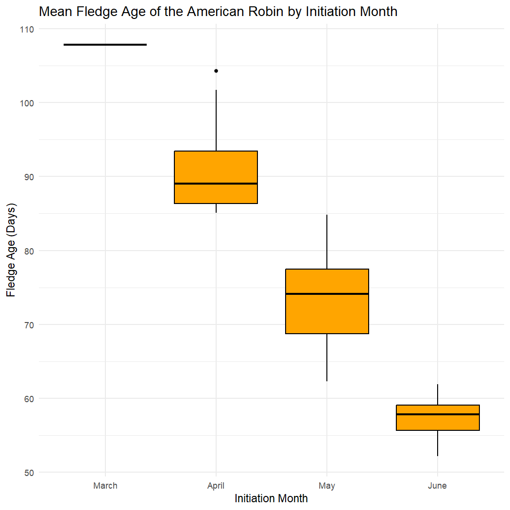

Boxplot represents the mean fledge age from each initiation month.

The mean fledge age for the American Robin appears to decrease with each subsequent initiation month.

2.6 rNest: Mapping

Let’s visualize some potential nesting patterns using the combined rNest and ecodistricts dataset. We can start by mapping the ecodistricts to compare fledging dates for the American Robin.

Convert the rnest_join dataframe to an sf object using the existing ‘geometry’ column

rnest_robin <- st_sf(rnest_robin)

Assign a Coordinate Reference System (CRS) like EPSG:4326 (WGS84) to the combined data.

rnest_robin <- st_transform(rnest_robin, crs = 4326)

Use ggplot() to visualize the Ecodistricts using a color ramp that represents fledging date.

# Plot ecodistricts with fledging date color ramp
ggplot() +
  geom_sf(data = rnest_robin, fill = "grey80", color = "white", size = 0.3) +  # Base ecodistrict map
  geom_sf(data = rnest_robin, aes(fill = fledging), color = "black", size = 0.2) + 
  scale_fill_viridis_c(option = "plasma", name = "Fledging Date") +  # Color ramp for fledging date
  labs(title = "Fledging Dates (Julian) by Ecodistrict for the American Robin",
       caption = "Source: rNest and National Ecological Framework for Canada") +
  theme_minimal() +
  theme(legend.position = "right")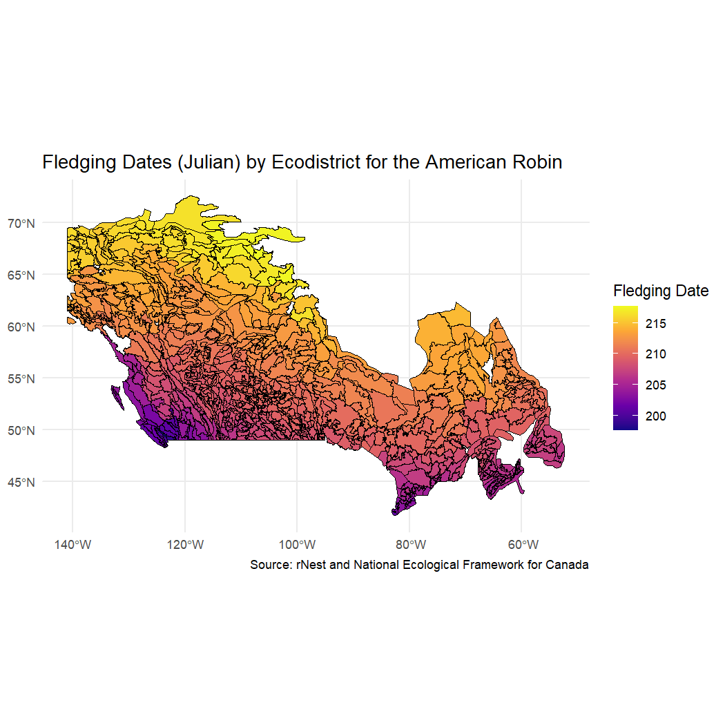

Map visualizes the ecodistricts by fledging data using a color ramp.

Congratulations! You completed Chapter 2: Auxiliary Tables. Here, you accessed NatureCounts auxiliary tables using the nc_query_tables function. You also created basic data summaries and maps using rNest and ecodistricts data.

Chapter 2 - Auxiliary Tables

2025-03-27