Chapter 1 - Zero-filling • naturecounts

Chapter 1: Zero-filling

Author: Dimitrios Markou, Steffi LaZerte, Danielle Ethier

Including both zero and non-zero counts is important to describe changes in bird distribution and abundance over time. Presence-only data offers limited information on these trends which can be affected by observer location bias and sampling effort. This chapter will cover three zero-filling methods and demonstrate how to produce presence/absence data for analysis.

This tutorial assumes that you have a basic understanding of how to access your data from NatureCounts. The NatureCounts Introductory R Tutorial is where you should start if you’re new to the naturecounts R package. It explains how to access, view, filter, manipulate, and visualize NatureCounts data. We recommend reviewing this tutorial before proceeding.

1.0 Learning Objectives

By the end of Chapter 1 - Zero-filling, users will know how to:

Determine if their data is suitable for zero filling: Intro to zero-filling
Zero-fill NatureCounts data and generate a presence/absence column: format_zero_fill function
Create an events data matrix to zero-fill data for select species: Events matrix
Run a for loop to zero-fill data for multiple species in sequence: Events matrix loop

This R tutorial requires the following packages:

library(naturecounts)
library(tidyverse)

1.1 Intro to Zero-filling

When observers are collecting point count data in the field, they are recording all the birds they see or hear. They are not recording the birds that they do not see or hear. NatureCounts data set therefore often lack zeros for species that were not detected during a survey. Zero-filling assigns a count of zero to species that are not detected during an observation period (ObservationCount = 0). Zeros can indicate two things - the true absence of a species or failure to detect a species.

Here are some important considerations to keep in mind when applying zero-filling methods:

Biological Relevance: Ensure that the zeros you are adding accurately reflect true absences rather than just missing data. This distinction is crucial for valid interpretations.
Sampling Bias: Consider potential biases in your sampling methods. If certain areas or times are under-sampled, zero-filling may misrepresent the actual distribution and abundance of species.
Data Structure: Understand the structure of your dataset. Zero-filling may be more appropriate for certain types of data (e.g., count data) than others (e.g., presence-only data).
Statistical Methods: Choose appropriate statistical methods that can handle zero-inflated data. Some models are specifically designed for datasets with many zeros, while others may not be suitable.
Impact on Analysis: Assess how zero-filling will affect your analysis outcomes. Adding zeros can influence mean values, variances, and other statistical metrics, potentially leading to misleading conclusions.
Documentation: Clearly document your zero-filling process, including the rationale for your chosen method and any assumptions made. This transparency is essential for reproducibility and for others to understand your analysis.
Contextual Factors: Take into account environmental or temporal factors that may influence species presence or absence. These factors can help inform whether zeros are appropriate in specific contexts.

By carefully considering these factors, you can make more informed decisions about zero-filling and its implications for your dataset and subsequent analyses.

Good candidates for zero-filling are species that are reported consistently at many sites within their ranges. What is considered “many sites” depends on the species. Species that are rarely detected or are considered outside of their range are likely poor candidates for zero-filling.

Note: Zero-filling, across all methods, assumes that at least one species was detected at each survey point. This assumption is nearly always true.

1.2 NatureCounts format_zero_fill function

The format_zero_fill() function can help us infer species absence when a species was not detected during a sampling event, provided that all species were reported for that event (i.e. AllSpeciesReported is “Yes”). Otherwise, the function will return an error for invalid records. If your dataset produces an error, you will need to filter your data to only SamplingEventIdentifiers where all species were recorded.

Browse the collections to find the Breeding Bird Surveys (BBS; 50 stops, Canada) dataset.

collections <- meta_collections()
View(meta_collections())

Let’s bring in the list of common names to append to the dataframe for easier interpretation.

sp.list <- search_species()
sp.list <- sp.list %>% dplyr::select(species_id, english_name)

Read in the BBS data from NatureCounts from 2015 to 2020 from the province of Saskatchewan as an example data set. Because we want to zero-fill the dataframe, we need to download the full collection for the given time period and geography of interest. NOT just the data for the species of interest. This will ensure that all the sampling events are correctly identified for zero-filling.

bbs50_can <- nc_data_dl(collections = "BBS50-CAN", years=c(2015,2020), region=list(statprov="SK"), username = "testuser", info = "zero fill example")

Append the english name to the BBS dataframe and ensure ObservationCount is numeric.

bbs50_can <- bbs50_can %>% left_join(sp.list, by = "species_id")
bbs50_can$ObservationCount <- as.numeric(bbs50_can$ObservationCount)

Determine if all species were reported in the dataset.

count(bbs50_can, AllSpeciesReported)
#>   AllSpeciesReported     n
#> 1                Yes 80385

Yes! So, in this case, there is no need to filter the dataset because all species were recorded for each sampling event.

Let’s apply the format_zero_fill() function. Optionally, you can specify columns to retain in the output dataframe using the extra_event and/or extra_species arguments. By default, the function zero fills by SamplingEventIdentifier. However, the by argument may also be used to specify how the data should be zero-filled i.e. by SamplingEventIdentifer, SurveyAreaIdentifier, SiteCode, utm_square, etc. This is useful if you want to determine whether a species has/has not been observed in a particular zone!

bbs50_can_zero_fill <- format_zero_fill(bbs50_can, 
                                 by = "SamplingEventIdentifier",
                                 extra_event = c("latitude", "longitude"),
                                 extra_species = "english_name")

While format_zero_fill() adds 0’s to the ObservationCount column by default, you can specify other columns to zero fill. For example, you could create Presence/Absence data by zero-filling a custom column.

First, select relevant columns from the original dataframe and create a presence column based on ObservationCount.

bbs50_can_presence <- bbs50_can %>%
  dplyr::select(AllSpeciesReported, SamplingEventIdentifier, species_id, ObservationCount, latitude, longitude, english_name) %>%
  mutate(presence = if_else(as.numeric(ObservationCount) > 0, TRUE, FALSE))

Zero-fill the data while specifying the presence column in the fill argument. This also converts the presence column from logical to numeric.

bbs50_can_pres_filled <- format_zero_fill(bbs50_can_presence, 
                                          fill = "presence",
                                          by = "SamplingEventIdentifier",
                                          extra_event = c("latitude", "longitude"), 
                                          extra_species = "english_name")
#>  - Converted 'fill' column (presence) from logical to numeric

1.3 Zero-filling: Events matrix

In some instances, you may have a survey that does not record all species (e.g., Nocturnal Owl Survey, Marsh Monitoring Program, Hawk Watch), but rather targeted species specific to the programs protocol. If AllSpeciesRecorded is not YES, you will want to zero-fill your dataframe based on an events matrix that specifies which sites were surveyed within a specific time frame and geography. This matrix lists all survey events that took place, regardless of how many or which species were observed.

To create the events matrix, we extract unique combinations of survey time (e.g., day, month, year, TimeObservationStarted, TimeObservationEnded) and location (SamplingAreaIdentifier, RouteIdentifier, SiteCode, latitude, longitude). Which variables you select will be specific to your analysis. Generally, the following variables from the NatureCounts BMDE work well:

events_matrix <- bbs50_can %>%
  dplyr::select(SiteCode,
         survey_year,
         survey_month,
         survey_day,
         latitude, 
         longitude) %>%
  distinct()

From this, you can see there are 9510 unique survey events in the BBS dataset from 2015-2020 in Saskatchewan.

Filter the NatureCounts data for a species of interest and then merge the events matrix with the species-specific data. This will result in NA values for events where the species was not observed.

search_species("Chestnut-collared Longspur") #species_id = 19160
#> # A tibble: 1 × 5
#>   species_id scientific_name   english_name               french_name                taxon_group
#>        <int> <chr>             <chr>                      <chr>                      <chr>      
#> 1      19160 Calcarius ornatus Chestnut-collared Longspur Plectrophane à ventre noir BIRDS

longspur_events <- bbs50_can %>%
  filter(species_id == "19610")

longspur_events <- left_join(events_matrix, longspur_events,
                          by = c("SiteCode",
                               "survey_year",
                               "survey_month",
                               "survey_day",
                               "latitude",
                               "longitude"))

Zero-fill for specific species. Here, we replace the NA values in the ObservationColumn with 0 and select the column of interest to inspect your data.

longspur_zero_fill <- longspur_events %>% 
  mutate(ObservationCount = replace(ObservationCount, is.na(ObservationCount), 0)) %>% dplyr::select(SiteCode, survey_day, survey_month, survey_year, latitude, longitude, ObservationCount)

Plot a histogram of your zero-filled observation counts of Chestnut-collared Longspur to see how the data are distributed.

hist(longspur_zero_fill$ObservationCount, breaks = 10)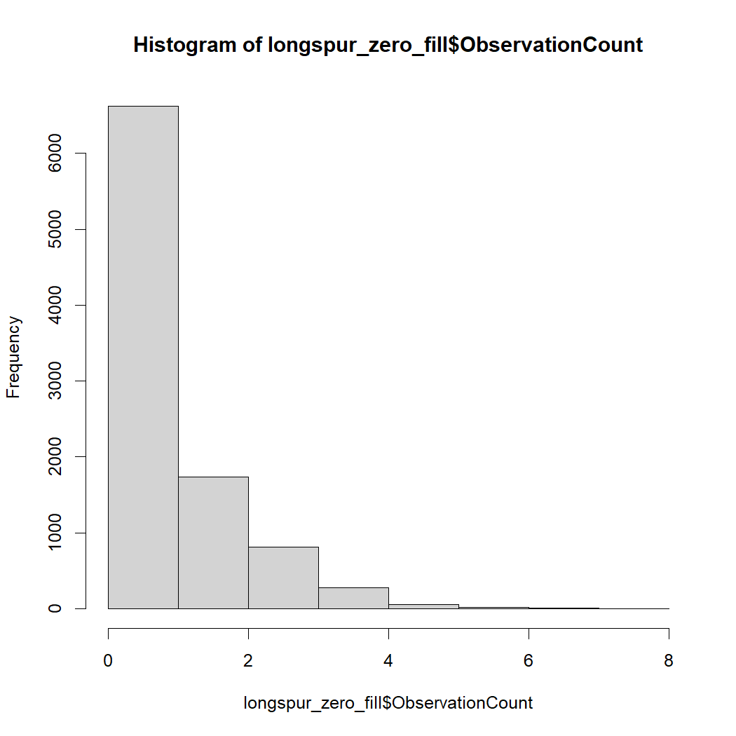

Plot shows histogram of zero-filled Chestnut-collared Longspur observation counts.

Now your data frame is zero filled. You can repeat this process for other species of interest or learn in the next section how to zero-fill multiple species in sequence using a loop.

1.4 Zero-filling: Events matrix loops

Oftentimes, when dealing with larger datasets, it might be more effective to zero-fill across several species in sequence using a loop.

for loops execute code until told to stop (i.e. for a specified number of iterations)
while loops execute code as long as a condition is met

First, extract the individual species_id values from the BBS dataset.

sp_ids <- unique(bbs50_can$species_id)

Optional: You can also create the list manually for just a handful of species of interest rather than all the species in the dataset. To execute the code chunk below, remove the #.

# sp_ids <- c(19160, 19170, 19180) # Chestnut-collared Longspur, Upland Sandpiper, Western Meadowlark

Next, initialize an empty list to store our zero-filled data and build the for loop step by step.

zero_filled_data <- list()

# Loop through each sp_ids
for (i in sp_ids) {
  # Filter the BBS data for each species in a given loop
  all_species_data <- bbs50_can %>% 
    filter(species_id == i)
  
  # Join the NatureCounts data with the events matrix
  all_species_events <- left_join(events_matrix, all_species_data,
                                  by = c("SiteCode", 
                                         "survey_year", 
                                         "survey_month",
                                         "survey_day", 
                                         "latitude", 
                                         "longitude"))
  
  # Zero-fill the `ObservationCount` column for each species and across all events
  all_species_events <- all_species_events %>%
    mutate(ObservationCount = replace(ObservationCount, is.na(ObservationCount), 0))
  
  # Add the result to the list with species_id as the key
  zero_filled_data[[as.character(i)]] <- all_species_events
}

We can then combine the results from the loop into a single dataframe which contains the zero-filled data for all species.

zero_filled_dataframe <- bind_rows(zero_filled_data, .id = "species_id")

Congratulations! You completed Chapter 1: Zero-filling. Here, you explored three methods for zero-filling observation counts and generated presence/absence data. For more examples on zero-filling, see this supplementary article. In Chapter 2, you can explore how to access auxiliary datatables in the NatureCounts database using the nc_query_table() function.

Chapter 1 - Zero-filling

2025-03-27