Chapter 1 - Spatial Data Exploration • naturecounts

Chapter 1: Spatial Data Exploration

Authors: Dimitrios Markou, Danielle Ethier

Exploring your data in a visual way is an important first step to any analysis. This chapter will give you a foundational understanding of how to work with your NatureCounts data spatially in R. This Chapter assumes that you have a basic understanding of how to access your data from NatureCounts. The NatureCounts Introductory R Tutorial is where you should start if you’re new to the naturecounts R package. It explains how to access, view, filter, manipulate, and visualize NatureCounts data. We recommend reviewing this tutorial before proceeding.

1.0 Learning Objectives

By the end of Chapter 1 - Spatial Data Exploration, users will know how to:

Distinguish between types of spatial data (vector vs raster)
Select from a variety of geoprocessing functions in the sf package
Visualize NatureCounts data using spatio-temporal maps

This R tutorial requires the following packages:

library(naturecounts)
library(sf)
library(dplyr)
library(ggplot2)
library(ggspatial)

1.1 Spatial Data Types

Spatial data is any type of vector or raster data that represents a feature or phenomena across geographic space.

Vector data is used to represent features with points, lines and polygons. This may include individual bird observations, rivers, or conservation area boundaries.

Raster data is used to represent spatially continuous data with a grid, where each cell has one value. This may include types of environmental data like temperature, elevation or land use.

The most common format used to store vector data in a file on disk is the ESRI Shapefile format (.shp). Shapefiles are always accompanied by files with .dbf, .shx, and .prj extensions.

Raster data files are typically stored with TIFF or GeoTIFF files with a (.tif) or (.tiff) extension. Raster data manipulation will be in covered in subsequent chapters (see Chapter 3: Climate Data, Chapter 4: Elevation Data, Chapter 5: Land Cover Data, Chapter 6: Satellite Imagery, and Chapter 7: Raster Summary).

Vector and raster data may also be associated with attribute data or temporal data. Attribute data provides additional information on the characteristics of spatial features while temporal data assigns a specific date or time range.

The sf package provides simple feature access in R. This package works best with spatial data (point, line, polygon, multipolygon) associated with tabular attributes (e.g shapefiles). You may be familiar with the sp package that has similar functionality in a different format, however, this package is no longer in use as of 2023 and does not support integration with tidyverse which is very popular among data scientists who use R.

1.2 Geo-processing Functions

Geoprocessing functions allow us to manipulate or compute spatial objects based on interactions between their geometries. There are several useful functions integrated into the sf package including:

st_transform() - transforms the CRS of a specified CRS object
st_drop_geometry() - removes the geometry column of a sf object
st_intersection(x, y) - creates geometry of the shared portion of x and y
st_crop(x, y, ..., xmin, ymin, xmax, ymax) - creates geometry of x that intersects a specified range
st_difference(x, y) - creates geometry from x that does not intersect with y
st_area, st_length, and st_distance can also be used to compute geometric measurements

More resources, including an sf package cheatsheat can be found here.

1.3 Spatio-temporal Mapping

Example 1 - You would like to visualize the spatio-temporal distribution of Cedar Waxwing observations in June of each survey year using data from the Maritimes Breeding Bird Atlas (2006-2010).

Let’s fetch the NatureCounts data.

First, we look to find the collection code for the Maritimes Breeding Bird Atlas.

collections <- meta_collections()
View(meta_collections())

Second, we look to find the numeric species id.

search_species("cedar waxwing")
#> # A tibble: 2 × 5
#>   species_id scientific_name              english_name           french_name                    taxon_group
#>        <int> <chr>                        <chr>                  <chr>                          <chr>      
#> 1      16330 Bombycilla cedrorum          Cedar Waxwing          Jaseur d'Amérique              BIRDS      
#> 2      40749 Bombycilla garrulus/cedrorum Bohemian/Cedar Waxwing Jaseur boréal ou J. d'Amérique BIRDS

Now we can download the data.

The data download will not work unless you replace "testuser" with your actual user name. You will be prompted to enter your password.

cedar_waxwing <- nc_data_dl(collections = "MBBA2PC", species = 16330, 
                            username = "testuser", info = "spatial_data_tutorial")
#> Using filters: collections (MBBA2PC); species (16330); fields_set (BMDE2.00-min)
#> Collecting available records...
#>   collection nrecords
#> 1    MBBA2PC     1659
#> Total records: 1,659
#> 
#> Downloading records for each collection:
#>   MBBA2PC
#>     Records 1 to 1659 / 1659

Use the format_dates function to create date and day-of-year (doy) columns.

cedar_waxwing <- format_dates(cedar_waxwing)

Filter the data to only include observations from the month of June.

cedar_waxwing_june <- cedar_waxwing %>%
  filter(survey_month == 6)

Convert the NatureCounts data to a spatial object using the point count coordinates.

cedar_waxwing_june_sf <- st_as_sf(cedar_waxwing_june,
                                  coords = c("longitude", "latitude"), crs = 4326)

Finally, use ggplot2 to visualize the spatio-temporal distribution of Cedar Waxwing observations across the Maritime provinces by color-coding the data points by survey_year and creating a multi-panel plot based on this discrete variable:

ggplot(data = cedar_waxwing_june_sf) +
  # Select a basemap
  annotation_map_tile(type = "cartolight", zoom = NULL, progress = "none") +
  # Plot the points, color-coded by survey_year
  geom_sf(aes(color = as.factor(survey_year)), size = 1) +
  # Facet by survey_year to create the multi-paneled map
  facet_wrap(~ survey_year) +
  # Customize the color scale
  scale_color_brewer(palette = "Set1", name = "Survey Year") +
  # Add a theme with a minimal design and change the font styles, to your preference
  theme_minimal() +
  theme(legend.position = "bottom") +
  # To make the points in the legend larger without affecting map points
  guides(color = guide_legend(override.aes = list(size = 3))) +
  # Define the title and axis names
  labs(title = "Cedar Waxwing June Observations by Survey Year",
       x = "Longitude",
       y = "Latitude")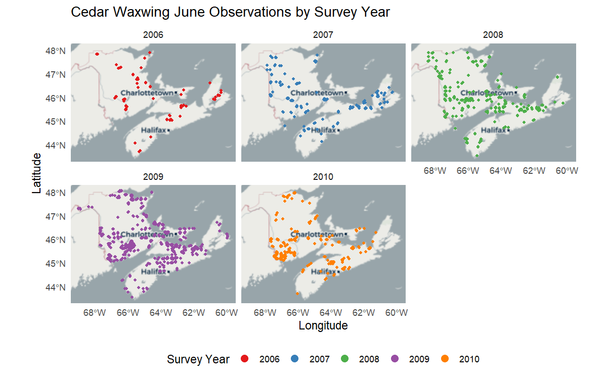

Five annual maps of Maritime Canada showing observations of cedar waxings 2006-2010

The map above provides a simple visualization of NatureCounts data over a broad spatial and temporal scale.

Congratulations! You completed Chapter 1: Spatial Data Exploration. Here, you successfully visualized NatureCounts vector data over a wide spatial and temporal scale using a multi-panel plot. In Chapter 2, you can explore spatial data manipulation, apply geoprocessing functions, and visualize NatureCounts data within Key Biodiversity Areas (KBAs) and Priority Places.

Chapter 1 - Spatial Data Exploration

2025-03-27