Chapter 2 - Spatial Subsetting • naturecounts

Chapter 2: Spatial Subsetting: KBA’s and Priority Places

Authors: Dimitrios Markou, Danielle Ethier

In Chapter 1: Spatial Data Exploration, you distinguished between spatial data types (vector and raster) and explored NatureCounts data using a spatio-temporal map. Now you are ready to focus your data exploration to a specific geographic area. Analyzing NatureCounts data within specific boundaries is relevant to many research application. Here we use Key Biodiversity Areas (KBA) and Priority Places as examples of research areas of interest.

2.0 Learning Objectives

By the end of Chapter 2 - Spatial Subsetting, users will know how to:

Import and map polygon boundary files based on attributes
Reproject NatureCounts data to the coordinate reference system of your spatial layer
Spatially filter and map NatureCounts data for an area of interest
Read, process, and visualize spatial vector data within areas of significant conservation potential: Key Biodiversity Areas (KBAs) and Priority Places for Species at Risk.

The data used in this tutorial are downloaded from NatureCounts, the KBA Canada Map Viewer, and the Priority Places - Open Government Portal. You will save the downloaded shapefiles to your working directory.

To view your working directory.

getwd()

This R tutorial requires the following packages:

library(naturecounts)
library(sf)
library(dplyr)
library(ggplot2)
library(ggspatial)
library(mapview)
library(leaflet)
library(leaflet.extras)

2.1 Key Biodiversity Areas

Example 2a - You are interested in assessing the spatial distribution of Wood Ducks (Ontario Breeding Bird Atlas data) across the KBAs found within the province of Ontario.

Navigate the the KBA Canada Map Viewer and filter the data for Ontario using the left hand Province/Territory filter. Then select ‘Download’. You will want to select both csv and shp for this example.

We can read in our KBA polygons using the sf package once it is in your working directory. The downloaded files was renamed for this example so you will need to change the code to match your file name.

ontario_kba <- st_read("ontario_kba.shp")

sf objects are stored in R as a spatial dataframe which contains the attribute table of the vector along with the geometry type. When we examine the dataframe, it looks like there are many duplicate entries including duplicate geometries (vertices). To clean this up, we can apply the st_make_valid() and distinct() functions to our spatial dataframe:

ontario_kba <- ontario_kba %>% st_make_valid() %>% distinct()

Our spatial data is also accompanied by a CSV file that contains additional useful attributes (landcover, species, etc) concerning our KBAs. Let’s read in the accompanying CSV file for our KBA layer.

kba_attributes <- read.csv("ontario_kba.csv")

Great! We can now join these dataframes using the handy tidyverse package. However, we’ll want to select for specific columns first to avoid redundancies before performing our join:

kba_attributes <- kba_attributes %>%
  select("SiteCode",
         "DateAssessed",
         "PercentProtected",
         "BoundaryGeneralized",
         "Level",
         "CriteriaMet",
         "ConservationActions",
         "Landcover",
         "Province",
         "Species")

Both dataframes now contain unique columns, after our selection. We apply the full_join() function to hold all attributes within one dataframe.

ontario_kba <- full_join(ontario_kba, kba_attributes, by = "SiteCode")

To visualize the ontario_kba data we can use ggplot().

ggplot() + 
  # Select the basemap
  annotation_map_tile(type = "cartolight", zoom = NULL, progress = "none") +
  # Add the polygon data
  geom_sf(data = ontario_kba, aes(fill = "Ontario KBAs"), color = "black", 
          size = 0.5, alpha = 0.5) +
  # Add the map components
  theme_minimal() + 
  scale_fill_manual(values = c("Ontario KBAs" = "red")) + 
  theme(legend.position = "bottom") +
  labs(title = "Key Biodiversity Areas (KBAs) of Ontario",
       x = "Longitude",
       y = "Latitude",
       fill = "Legend")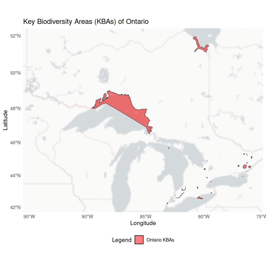

Map showing key biodiversity areas in Ontario, outlined in pink

We can also visualize the ontario_kba data with an interactive map, using the leaflet package.

leaflet(width = "100%") %>%
  addTiles() %>%
  addPolygons(data = ontario_kba, color = "black", weight = 2, smoothFactor = 1, 
              opacity = 1.0, fillOpacity = 0.5, fillColor = "red") %>% 
  addFullscreenControl() %>%
  addLegend(colors = c("red"),labels = c("Ontario KBAs"), position = "bottomright")

Similarly, the package mapview (based on leaflet) can be used to make interactive plots. We can represent specific attributes like so:

mapview(ontario_kba, zcol = "PercentProtected")

In this example, were interested in all the KBA polygons of Ontario. However, if you were working with a larger data set, it is possible to filter your dataframe to retrieve only specific polygons that meet certain criteria relevant to your research. To do so, we can apply filters based on a variable condition. For example, say we only wanted KBA’s greater than 100km^2 in size:

To execute this code chunk, remove the #

# kba_name <- ontario_kba %>% 
  # filter(Area > 100)

Let’s search NatureCounts for the Ontario Breeding Bird Atlas point count dataset using meta_collections() and the Wood Duck species ID using search_species().

collections <- meta_collections()
View(meta_collections())

search_species("wood duck")
#> # A tibble: 5 × 5
#>   species_id scientific_name                    english_name                          french_name                           taxon_group
#>        <int> <chr>                              <chr>                                 <chr>                                 <chr>      
#> 1        360 Aix sponsa                         Wood Duck                             Canard branchu                        BIRDS      
#> 2      40938 Aix sponsa x Anas platyrhynchos    Wood Duck x Mallard (hybrid)          Hybride Canard branchu x C. colvert   BIRDS      
#> 3      41197 Aix sponsa x Lophodytes cucullatus Wood Duck x Hooded Merganser (hybrid) Hybride Canard branchu x Harle couro… BIRDS      
#> 4      45989 Aix sponsa x Mareca americana      Wood Duck x American Wigeon (hybrid)  Hybride Canard branchu x C. d'Amériq… BIRDS      
#> 5      47173 Tadorna tadorna x Aix sponsa       Common Shelduck x Wood Duck (hybrid)  Hybride Tadorne de Belon x Canard br… BIRDS

Now we can download the NatureCounts data. Remember to change testuser to your personal username.

atlas_on <- nc_data_dl(collections = "OBBA2PC", species = 360, 
                       username = "testuser", info = "spatial_data_tutorial")

We can then convert our NatureCounts data into a spatial object. To do so, we deploy the st_as_sf function and specify the coordinate reference system (CRS).

The CRS of our KBA sf object can be returned with st_crs().

st_crs(ontario_kba)
#> Coordinate Reference System:
#>   User input: WGS 84 
#>   wkt:
#> GEOGCRS["WGS 84",
#>     DATUM["World Geodetic System 1984",
#>         ELLIPSOID["WGS 84",6378137,298.257223563,
#>             LENGTHUNIT["metre",1]]],
#>     PRIMEM["Greenwich",0,
#>         ANGLEUNIT["degree",0.0174532925199433]],
#>     CS[ellipsoidal,2],
#>         AXIS["latitude",north,
#>             ORDER[1],
#>             ANGLEUNIT["degree",0.0174532925199433]],
#>         AXIS["longitude",east,
#>             ORDER[2],
#>             ANGLEUNIT["degree",0.0174532925199433]],
#>     ID["EPSG",4326]]

Our KBA sf object is stored with World Geodetic System 1984 (WGS 84) coordinates, EPSG = 4326. Now we can convert our atlas_on dataframe to an sf object using the same CRS.

atlas_on_sf <- st_as_sf(atlas_on,
                        coords = c("longitude", "latitude"), crs = 4326)

Now let’s ensure that the conversion was successful. You’ll notice a new geometry column where each observation is a point.

str(atlas_on_sf) # view the sf object
#> Classes 'sf' and 'data.frame':   290 obs. of  56 variables:
#>  $ record_id              : int  10339750 10340180 10342681 10343644 10344845 10351428 10353184 10354352 10355078 10357496 ...
#>  $ collection             : chr  "OBBA2PC" "OBBA2PC" "OBBA2PC" "OBBA2PC" ...
#>  $ project_id             : int  1007 1007 1007 1007 1007 1007 1007 1007 1007 1007 ...
#>  $ protocol_id            : logi  NA NA NA NA NA NA ...
#>  $ protocol_type          : int  1 1 1 1 1 1 1 1 1 1 ...
#>  $ species_id             : int  360 360 360 360 360 360 360 360 360 360 ...
#>  $ statprov_code          : chr  "ON" "ON" "ON" "ON" ...
#>  $ country_code           : chr  "CA" "CA" "CA" "CA" ...
#>  $ SiteCode               : chr  "17NJ64-14" "17MJ97-10" "17NH47-23" "17NJ31-6" ...
#>  $ bcr                    : int  13 13 13 13 13 13 13 12 13 13 ...
#>  $ subnational2_code      : chr  "CA.ON.WL" "CA.ON.BC" "CA.ON.BN" "CA.ON.WT" ...
#>  $ iba_site               : chr  "N/A" "N/A" "N/A" "N/A" ...
#>  $ utm_square             : chr  "17TNJ64" "17TMJ97" "17TNH47" "17TNJ31" ...
#>  $ survey_year            : int  2001 2001 2001 2001 2001 2001 2001 2001 2001 2001 ...
#>  $ survey_month           : int  6 5 5 6 6 6 6 6 6 6 ...
#>  $ survey_week            : int  3 4 4 3 1 4 4 1 4 2 ...
#>  $ survey_day             : int  21 31 31 24 4 28 28 2 27 15 ...
#>  $ breeding_rank          : logi  NA NA NA NA NA NA ...
#>  $ GlobalUniqueIdentifier : chr  "URN:catalog:BSC-EOC:OBBA2PC:850-WODU" "URN:catalog:BSC-EOC:OBBA2PC:392-WODU" "URN:catalog:BSC-EOC:OBBA2PC:269-WODU" "URN:catalog:BSC-EOC:OBBA2PC:961-WODU" ...
#>  $ CatalogNumber          : chr  "850-WODU" "392-WODU" "269-WODU" "961-WODU" ...
#>  $ Locality               : logi  NA NA NA NA NA NA ...
#>  $ TimeCollected          : chr  "5.7166667" "8.9333334" "7.1999998" "6.2833333" ...
#>  $ CollectorNumber        : chr  "356" "266" "1530" "1335" ...
#>  $ FieldNumber            : logi  NA NA NA NA NA NA ...
#>  $ Remarks                : logi  NA NA NA NA NA NA ...
#>  $ ProjectCode            : chr  "OBBA2" "OBBA2" "OBBA2" "OBBA2" ...
#>  $ ProtocolType           : chr  "Point Count" "Point Count" "Point Count" "Point Count" ...
#>  $ ProtocolCode           : chr  "PointCount" "PointCount" "PointCount" "PointCount" ...
#>  $ ProtocolURL            : chr  "http://www.bsc-eoc.org/norac/atlascont.htm" "http://www.bsc-eoc.org/norac/atlascont.htm" "http://www.bsc-eoc.org/norac/atlascont.htm" "http://www.bsc-eoc.org/norac/atlascont.htm" ...
#>  $ SurveyAreaIdentifier   : chr  "17NJ64-14" "17MJ97-10" "17NH47-23" "17NJ31-6" ...
#>  $ SamplingEventIdentifier: chr  "850" "392" "269" "961" ...
#>  $ SamplingEventStructure : logi  NA NA NA NA NA NA ...
#>  $ RouteIdentifier        : chr  "17NJ64" "17MJ97" "17NH47" "17NJ31" ...
#>  $ TimeObservationsStarted: logi  NA NA NA NA NA NA ...
#>  $ TimeObservationsEnded  : logi  NA NA NA NA NA NA ...
#>  $ DurationInHours        : chr  "0.08333333" "0.08333333" "0.08333333" "0.08333333" ...
#>  $ TimeIntervalStarted    : chr  "5.7166667" "8.9333334" "7.1999998" "6.2833333" ...
#>  $ TimeIntervalEnded      : logi  NA NA NA NA NA NA ...
#>  $ TimeIntervalsAdditive  : logi  NA NA NA NA NA NA ...
#>  $ NumberOfObservers      : logi  NA NA NA NA NA NA ...
#>  $ NoObservations         : logi  NA NA NA NA NA NA ...
#>  $ ObservationCount       : chr  "2" "1" "1" "3" ...
#>  $ ObservationDescriptor  : chr  "Total count" "Total count" "Total count" "Total count" ...
#>  $ ObservationCount2      : chr  NA "1" NA "3" ...
#>  $ ObservationDescriptor2 : chr  "0-100 m" "0-100 m" "0-100 m" "0-100 m" ...
#>  $ ObservationCount3      : chr  "2" NA "1" NA ...
#>  $ ObservationDescriptor3 : chr  ">100 m" ">100 m" ">100 m" ">100 m" ...
#>  $ ObservationCount4      : logi  NA NA NA NA NA NA ...
#>  $ ObservationDescriptor4 : logi  NA NA NA NA NA NA ...
#>  $ ObservationCount5      : logi  NA NA NA NA NA NA ...
#>  $ ObservationDescriptor5 : logi  NA NA NA NA NA NA ...
#>  $ ObservationCount6      : logi  NA NA NA NA NA NA ...
#>  $ ObservationDescriptor6 : logi  NA NA NA NA NA NA ...
#>  $ AllIndividualsReported : chr  "Yes" "Yes" "Yes" "Yes" ...
#>  $ AllSpeciesReported     : chr  "Yes" "Yes" "Yes" "Yes" ...
#>  $ geometry               :sfc_POINT of length 290; first list element:  'XY' num  -80.1 43.7
#>  - attr(*, "sf_column")= chr "geometry"
#>  - attr(*, "agr")= Factor w/ 3 levels "constant","aggregate",..: NA NA NA NA NA NA NA NA NA NA ...
#>   ..- attr(*, "names")= chr [1:55] "record_id" "collection" "project_id" "protocol_id" ...

The st_transform() function can be applied to project our spatial object using a different CRS like NAD83 / UTM zone 16N (EPSG = 26916).

ontario_kba <- st_transform(ontario_kba, crs = 26916)

It can also be used to ensure that the CRS of our spatial objects match.

atlas_on_sf <- st_transform(atlas_on_sf, crs = st_crs(ontario_kba))

To identify Wood Ducks observed across Ontario KBA’s, we can apply the st_intersection() function.

wood_ducks_kba <- st_intersection(ontario_kba, atlas_on_sf)
#> Warning: attribute variables are assumed to be spatially constant throughout all geometries

You will get a warning message, which you can safely ignore.

# If need be, transform your spatial data back to EPSG:4326 to visualize with leaflet
ontario_kba <- st_transform(ontario_kba, crs = 4326)
wood_ducks_kba <- st_transform(wood_ducks_kba, crs = 4326)

Using ggplot, we can visualize the polygon data and point data.

ggplot() +
  # Select a basemap
  annotation_map_tile(type = "osm", zoom = NULL, progress = "none") +
  # Plot the filtered KBA polygon (ON001)
  geom_sf(data = ontario_kba, aes(fill = "Ontario KBA"), color = "black", size = 0.5, alpha = 0.5) +
  # Plot the Wood Duck observations that are within the KBA
  geom_sf(data = wood_ducks_kba, aes(color = "Wood Duck Observations"), size = 3, alpha = 0.8) +
  # Custom fill and color for the legend
  scale_fill_manual(values = c("Ontario KBA" = "violet"), name = "Legend") +
  scale_color_manual(values = c("Wood Duck Observations" = "orange"), name = "Legend") +
  # Automatically zoom to the extent of the ON001 polygon
  coord_sf() +
  # Map components
  theme_minimal() +
  theme(legend.position = "bottomright") +
  labs(title = "Key Biodiversity Area (KBA) - Long Point Peninsula and Marshes",
       x = "Longitude",
       y = "Latitude")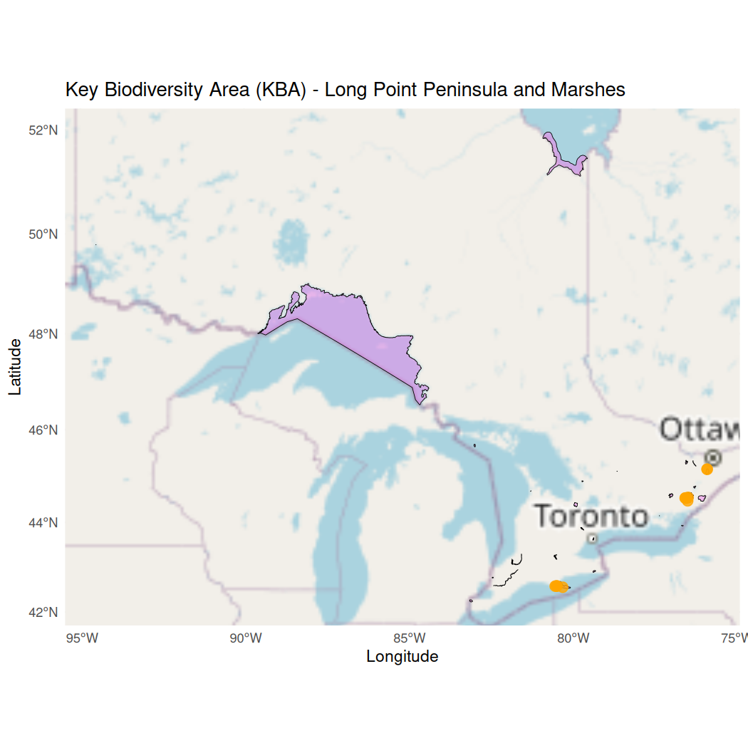

Map showing key biodiversity areas in Ontario, outlined in pink

You can also apply leaflet to visualize the polygon data and point data, using the addPolygons() addCircleMarkers() arguments.

leaflet(width = "100%") %>%
  addTiles() %>%
  addPolygons(data = ontario_kba, color = "black", weight = 2, smoothFactor = 1, 
              opacity = 1.0, fillOpacity = 0.5, fillColor = "violet") %>%
  addCircleMarkers(data = wood_ducks_kba, radius = 3, color = "orange", 
                   stroke = FALSE, fillOpacity = 0.8) %>%
  addFullscreenControl() %>%
  addLegend(colors = c("violet", "orange"), 
            labels = c("Ontario KBA", "Wood Duck Observations"), 
            position = "bottomright")

After geoprocessing our data, we can write out any sf objects to Shapefiles on a disk, where the argument delete_layer = TRUE is used to overwrite an existing file.

To execute this code chunk, remove the #

# st_write(wood_ducks_kba,"wood_ducks_kba.shp", driver = "ESRI Shapefile", delete_layer = TRUE)

2.2 Priority Places

Example 2b - You want to assess the spatial distribution of Wood Ducks (Ontario Breeding Bird Atlas data) across the Long Point Walsingham Forest Priority Place.

Navigate to Priority Places - Open Government Portal. Scroll down to the Data and Resources section and select the Priority Places file labeled English, dataset, and FGDB/GDB.

First, lets create a path to our downloaded Priority Place file.

gdb_path <- "PriorityPlaces.gdb"

Then, let’s inspect the spatial data.

gdb_layers <- st_layers(gdb_path)
print(gdb_layers)
#> Driver: OpenFileGDB 
#> Available layers:
#>               layer_name geometry_type features fields                     crs_name
#> 1 PriorityPlacesBoundary Multi Polygon       11     11 NAD83 / Canada Atlas Lambert
#> 2  PriorityPlacesProject   Multi Point       89     13 NAD83 / Canada Atlas Lambert

To read in our spatial data object, we apply the st_read function and specify our desired data layer.

priori_place_polygons <- st_read(dsn = gdb_path, layer = "PriorityPlacesBoundary")
#> Reading layer `PriorityPlacesBoundary' from data source 
#>   `/home/steffi/Projects/Business/Birds Canada/NatureCounts/naturecounts/misc/data/priority_places/priorityplaces.gdb' 
#>   using driver `OpenFileGDB'
#> Simple feature collection with 11 features and 11 fields
#> Geometry type: MULTIPOLYGON
#> Dimension:     XY
#> Bounding box:  xmin: -2135754 ymin: -586679 xmax: 2450963 ymax: 2554209
#> Projected CRS: NAD83 / Canada Atlas Lambert

Were interested in the spatial distribution of Wood Ducks across the Long Point Walsingham Forest Priority Place. We’ll filter based on a variable condition.

long_point_polygon <- priori_place_polygons %>%
  filter(Name == "Long Point Walsingham Forest") # filters based on multipolygon name

Then reproject the Wood Duck data to match our Priority Place using st_transform.

atlas_on_sf <- st_transform(atlas_on_sf, crs = st_crs(long_point_polygon))

Next, we’ll apply our geoprocessing function to find the Wood Duck observations that intersect with our chosen Priority Place.

wood_ducks_longpoint <- st_intersection(long_point_polygon, atlas_on_sf)
#> Warning: attribute variables are assumed to be spatially constant throughout all geometries

Finally, we’ll transform our spatial objects one more time before visualizing them with leaflet.

long_point_polygon <- st_transform(long_point_polygon, crs = 4326)
wood_ducks_longpoint <- st_transform(wood_ducks_longpoint, crs = 4326)

Use ggplot to visualize the polygon and point data.

ggplot() +
  # Select a basemap
  annotation_map_tile(type = "cartolight", zoom = NULL, progress = "none") +
  # Plot the Long Point polygon
  geom_sf(data = long_point_polygon, aes(fill = "Long Point Walsingham Forest"),  
          color = "black", size = 0.5, alpha = 0.5) +
  # Plot the Wood Duck observations
  geom_sf(data = wood_ducks_longpoint, aes(color = "Wood Duck Observations"), 
          size = 3, alpha = 0.8) +
  # Custom fill and color for the legend
  scale_fill_manual(values = c("Long Point Walsingham Forest" = "red"), name = "Legend") +
  scale_color_manual(values = c("Wood Duck Observations" = "green"), name = "Legend") +
  # Automatically zoom to the extent of the Long Point polygon
  coord_sf() +
  # Map components
  theme_minimal() +
  theme(legend.position = "bottomright") +
  labs(title = "Wood Duck Observations within Long Point Walsingham",
       x = "Longitude",
       y = "Latitude")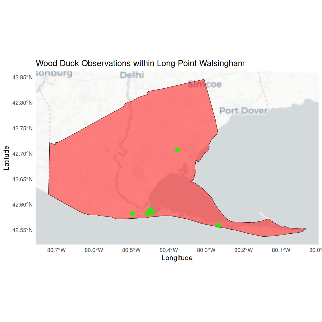

Map showing key biodiversity areas in Ontario, outlined in pink

You can also apply leaflet to visualize our polygon data and point data, using the addPolygons() addCircleMarkers() arguments.

leaflet(width = "100%") %>%
  addTiles() %>%
  addPolygons(data = long_point_polygon, color = "black", weight = 2, 
              smoothFactor = 1, opacity = 1.0, fillOpacity = 0.5, fillColor = "red") %>%
  addCircleMarkers(data = wood_ducks_longpoint, radius = 5, color = "green", 
                   stroke = FALSE, fillOpacity = 0.8) %>%
  addFullscreenControl() %>%
  addLegend(colors = c("red", "green"), 
            labels = c("Long Point Walsingham Forest", "Wood Duck Observations"), 
            position = "bottomright")

After geoprocessing our data, we can write out any sf objects to Shapefiles on a disk, where the argument delete_layer = TRUE is used to overwrite an existing file.

To execute this code chunk, remove the #

# st_write(wood_ducks_longpoint,"wood_ducks_longpoint.shp", driver = "ESRI Shapefile", delete_layer = TRUE)

Congratulations! You completed Chapter 2 - Spatial Subsetting: KBA’s and Priority Places. Here, you spatially filtered and visualized NatureCounts data. In Chapter 3, you can explore more spatial data visualization while linking climate data to NatureCounts observations.

Chapter 2 - Spatial Subsetting

2025-04-02

Chapter 2: Spatial Subsetting: KBA’s and Priority Places

Authors: Dimitrios Markou, Danielle Ethier

2.0 Learning Objectives

2.1 Key Biodiversity Areas

Example 2a - You are interested in assessing the spatial distribution of Wood Ducks (Ontario Breeding Bird Atlas data) across the KBAs found within the province of Ontario.

2.2 Priority Places

Example 2b - You want to assess the spatial distribution of Wood Ducks (Ontario Breeding Bird Atlas data) across the Long Point Walsingham Forest Priority Place.